In Depth – The Global Atmospheric Circulation

Global Atmospheric Circulation

One part of the Earth’s surface is always facing the Sun – it varies between the Tropic of Cancer at the June solstice to the Tropic of Capricorn at the December solstice.

This latitude receives the most energy per unit surface area, and is known as the Inter-Tropical Convergence Zone or ITCZ. Here, the air rises, hits the top of the troposphere and spreads out towards the poles. The Coriolis Effect means that this poleward moving air is deflected ever more to the right, becoming westerly (remember we name winds by the direction they are blowing from) and eventually sinking in the sub-tropics and returning towards the ITCZ – this time becoming easterly and giving us the Trade Winds. The whole circulation is known as the Hadley Cell (Figure 1).

FIGURE 1: A CROSS SECTION THROUGH THE ATMOSPHERE, SHOWING AIR RISING AND FORMING DEEP CLOUDS, AT THE INTERTROPICAL CONVERGENCE ZONE AND SPREADING POLEWARDS, AND THE HADLEY, FERREL AND POLAR CELLS.

Similarly, at the poles where the ground surface is coldest, the air sinks, spreads out towards the Tropics, is deflected to the right and eventually rises and completes a circulation – the Polar Cell.

In between, lies the ‘Ferrel cell’, characterised by surface westerlies and rising motion around 60°. This cell is actually the net product of all the mid-latitude weather systems. Figure 2 shows the 3-Dimensional circulation of the atmosphere.

It’s worth noting that, if the Earth wasn’t rotating, we’d have just one ‘thermally direct’ cell with air rising at the ITCZ and sinking at the poles where the ground is coldest.

The polar and sub-tropical High pressure areas are the source regions for air masses.

Teaching Resources

Global atmospheric circulation from Weather and Climate: a Teachers’ Guide.

Data and Image Sources

Take a look at the current air flow on the surface of the Earth, can you make out the Trade Winds? Do they tend to be stronger over land or ocean? Where is the ITCZ at the moment?

Global Atmospheric Circulation and Precipitation

  1. Visit https://svs.gsfc.nasa.gov/4285 and play the animation showing most currently available global precipitation data.
  2. Look at the map below. Circle any patterns of rainfall that you see.
Global precipitation map

3. What is the type of land is below these rainfall patterns? (Green is forest, brown is desert).                                                                                                                                                                                                                                    

4. In what latitude bands are these rainfall patterns?                                                                                                                                                            

Use these terms to fill in the blanks below for Questions 5-8: Hadley, cloud, humid, Sun, cloud, rainfall, low, ground, Ferrel, fronts, Equator, Hadley, poles, rainfall.

5. Rainfall occurs when ______ air cools down. Air cools when it rises, or when it moves away from the _______.

6. The Atmospheric Circulation is driven by the _____. In the Tropics, the Sun warms the _____ which in turn warms the air above. hot air rises, leading to _____ and _______. This drives the ________ cells.

7. Colder air sinks at the poleward edge of the _______ cells and over the __________. Sinking air has no _______ or __________.

8. In the _______ Cells, rainfall is mainly associated with ____ pressure systems (depressions). Rainfall is mainly on the ________.

9. Complete the following table (Look at the map for help):


Tropics

Sub Tropics

Poles

Skies

Clear/ Cloudy

Clear/ Cloudy

Clear/ Cloudy

Rain (or snow)-fall

Dry/ Wet

Dry/ Wet

Dry/ Wet

Pressure

High/ Low

High/ Low

High/ Low

10. Sketch what you think the Hadley Cell looks like in December and June by the images of the Earth below. Hint: the Equator and Tropics of Cancer and Capricorn are shown on the map.

Earth
Earth

Visit https://earth.nullschool.net/#current/wind/surface/level/overlay=precip_3hr/orthographic to see today’s rainfall patterns. Click on ‘Earth’ and then choose in the Overlay settings ‘3HPA’ to see the rainfall patterns together with surface wind speeds. Change in the settings the ‘Control’ to change the date and see rainfall patterns over time. Compare January and July rainfall patterns.

11. In the Tropics, how does the latitude of highest rainfall change between January and July?                                                                                                                                                                                                          ___________________________________                         

12. How does this relate to the sketches you drew above? ___________________________________________________________________________________________________________________________________________________________________________________________________________________________________________________

Extension question: Why do you think you are asked to look at rainfall in January and July, rather than December and June? ___________________________________________________________________________________________________________________________________________________________________________________________________________________________________________________

Rubber Ducks: an Unexpected Journey

1. Visit https://www.youtube.com/watch?v=_uuMpVf2R8E

2. On 10th January 1992 some 28,800 plastic bath-tub toys splashed into the sea at 44.7°N, 178.1°E. The first ducks arrived on beaches near Sitka in Alaska in September the same year, and then again in 1994, 1998, 2001, and 2003. The bath toys are still washing ashore today.

3. What does this tell us about the oceans?__________________________________________________________________________________________________________________________________________________________________________________________________________________________________________________________________________________________

4. Complete this table using the rubber ducks on the map, to show where each rubber duck has travelled to and which rubber duck made landfall first.

 Date of landfall Location of landfall Journey of rubber duck (oceans travelled through, countries passed by)


Extension: Using a map of the world’s ocean currents, identify which currents the ducks travelled on to reach their final destinations. 

5. What do the journeys of the rubber ducks tell you about ocean currents?__________________________________________________________________________________________________________________________________________________________________________________________________________________________________________________________________________________________

6. Why do you think the toys have been able to survive in the oceans since 1992?__________________________________________________________________________________________________________________________________________________________________________________________________________________________________________________________________________________________

7. Visit https://theoceancleanup.com/great-pacific-garbage-patch/ and watch the video and answer the following questions.

8. What is the Great Pacific Garbage Patch?__________________________________________________________________________________________________________________________________________________________________________________________________________________________________________________________________________________________

9. How much plastic floats in the Great Pacific Garbage Patch?________________________________________________________________________________________________________________________________________________________________

10. What are the effects on marine life and humans?__________________________________________________________________________________________________________________________________________________________________________________________________________________________________________________________________________________________

11. Do you think some of the Rubber Ducks might still be in the Great Pacific Garbage Patch? Why?__________________________________________________________________________________________________________________________________________________________________________________________________________________________________________________________________________________________


Global Atmospheric Circulation

Use this Global Atmospheric Circulation practice exercise.

Changes to the Global Atmospheric Circulation as the climate changes.

Other Useful Links

4. Atmospheric and Oceanic Circulation

Weather and Climate: a Teachers’ Guide

Pathway: Basic Weather, Climate 

Weather in our LivesWeather MeasurementsWeather and Climate – Atmospheric and Oceanic Circulation

Lesson overviewIn this lesson we look at the pattern of circulation of the atmosphere and oceans, driven by the Sun.


What makes the whole atmosphere rotate and move? What gives us defined areas where it is generally dry or rainy, warm or cold, high pressure or low pressure? The answer to all these questions ultimately lies in the fact that we live on a spherical rotating planet, at some distance from the Sun. The incident energy from the Sun is unequally distributed between the Tropics and the Poles, with the precise patterns changing through the year. The Earth’s atmosphere and oceans are in constant motion to redistribute heat. Although temperature differences ultimately drive this, the patterns of circulation are influenced by the planet’s rotation and topography.

Learning objectives:

  • To understand why different parts of the world receive different amounts of energy from the Sun.
  • To understand how that difference in energy received by the Earth causes air and ocean water to move from equatorial regions to the poles. 
  • To be able to describe key features of how the air and water move around the globe.

Key Teaching Resources

Atmospheric and Oceanic Circulation PowerPoint
Atmospheric and Oceanic Circulation PowerPoint (easier)
Atmospheric Circulation Worksheet
Atmospheric Circulation Worksheet (easier)
Atmospheric Circulation Homework
Board Game

Teacher CPD/ Extended Reading

Global Atmospheric and Oceanic Circulation – More for Teachers

Alternative or Extension Resources


Rubber Ducks – An Unexpected Journey – Explore what the dispersion of a cargo of rubber ducks tells us about the ocean circulation.


Weather and Climate: a Teachers’ Guide

Atmosphere

The Atmosphere

Origin of the atmosphere

The vertical structure of the atmosphere

Unequal heating of the Earth’s surface

Transfer of energy

Atmospheric cells

Synoptic features

Questions

Origin of the atmosphere

Definition and history of the Earth’s atmosphere

An atmosphere is defined as the gaseous envelope that surrounds a celestial body. Therefore, the Earth, like other planets in the solar system, has an atmosphere, which is retained by gravitational attraction and largely rotates with it.

Compared with the radius of the Earth, its atmosphere is very thin. 99% of the mass of the atmosphere lies below 30 km, or 0.5% of the equatorial radius.

Meteorology is the subject that studies the chemical and physical properties of the atmosphere together with its fields of motion, mass and moisture.

At the time of the Earth’s formation around 4.5 billion years ago there was probably no atmosphere. It is believed to have come into existence as a result of the volcanic expulsion of substances from its interior, ejecting mainly water vapour, with some carbon dioxide, nitrogen and sulphur. The atmosphere can only hold a certain amount of water vapour, so the excess condensed into liquid water to form the oceans.

It is thought that the first stage in the evolution of life, around 4,000,000,000 years ago, required an oxygen-free environment. At a later date, primitive forms of plant life developed in the oceans and began to release small amounts of oxygen into the atmosphere as a waste product from the cycle of photosynthesis, as shown by the following equation.

H2O + CO2 + sunlight → sugar + O2

This build-up of atmospheric oxygen eventually led to the formation of the ozone layer. This layer, approximately 8 to 30 km above the surface, helps to filter the ultraviolet portion of the incoming solar radiation spectrum. Therefore, as levels of harmful ultraviolet radiation decreased, so plants were able to move to progressively higher levels in the oceans.

This helped to boost photosynthesis and thereby the production of oxygen. Today, this element has reached levels where life has been sustainable on the surface of the planet through its presence, and it should be remembered that oxygen is an element which is not commonly found in the universe.

The composition of the atmosphere

The atmosphere is well mixed below 100 km, and apart from its highly variable water vapour and ozone contents, its composition is as shown below, excluding solid and liquid matter in suspension (aerosols).

COMPOSITION OF THE ATMOSPHERE
Gas
Symbol
% by weight
% by volume
Nitrogen
N2
75.52
78.09
Oxygen
O2
23.15
20.95
Argon
A
1.28
0.93
Carbon dioxide
CO2
0.046
0.035
Neon
Ne
0.012
0.0018
Helium
He
0.0007
0.0005
Methane
CH4
0.0008
0.00015
Krypton
Kr
0.003
0.0001
Ozone
O3
0-0.01
Variable
Water vapour
H20
0-4
Variable

The vertical structure of the atmosphere

The Earth’s atmosphere is most commonly divided into four isothermal layers or ‘spheres’: troposphere, stratosphere, mesosphere and thermosphere.

Fig 1: Vertical temperature profile of the ICAO Standard Atmosphere

Each layer is characterised by a uniform change in temperature with increasing altitude. In some layers there is an increase in temperature with altitude, whilst in others it decreases with increasing altitude. The top or boundary of each layer is denoted by a ‘pause’ where the temperature profile abruptly changes, as shown in Figure 1.

Troposphere

The troposphere contains about 80% of the atmosphere and is the part of the atmosphere in which we live, and make weather observations. In this layer, average temperatures decrease with height. This is known as adiabatic cooling, i.e. a change in temperature caused by a decrease in pressure. Even so, it is still more prone to vertical mixing by convective and turbulent transfer, than other parts of the atmosphere. These vertical motions and the abundance of water vapour make it the home of all important weather phenomena.

The troposphere’s thermal profile is largely the result of the heating of the Earth’s surface by incoming solar radiation. Heat is then transferred up through the troposphere by a combination of convective and turbulent transfer. This is in direct contrast with the stratosphere, where warming is the result of the direct absorption of solar radiation.

The troposphere is around 16 km high at the equator, with the temperature at the tropopause around -80 °C. At the poles, the troposphere reaches a height of around 8 km, with the temperature of the tropopause around -40 °C in summer and -60 °C in winter.

Therefore, despite the higher surface temperatures, the tropical tropopause is much cooler than at the poles.

Stratosphere

In contrast to the troposphere, temperatures in the stratosphere rise with increasing altitude. Another distinctive feature of the stratosphere is the absorption of ultraviolet radiation by ozone (O3). This is greatest around 50 km, which is where the stratopause occurs. Temperatures reach a maximum here, and according to latitude and season, they range from -30 °C over the winter pole to +20 °C over the summer pole.

As well as a noticeable change in temperature, the move from the troposphere into the stratosphere is also marked by an abrupt change in the concentrations of the variable trace constituents. Water vapour decreases sharply, whilst ozone concentrations increase. These strong contrasts in concentrations are a reflection of little mixing between the moist, ozone-poor troposphere and the dry, ozone-rich stratosphere.

Despite the dryness of the stratosphere, some clouds have developed in winter months over high latitudes at altitudes between 17 and 30 km, stretching into the stratosphere. They generally display iridescence and are known as nacreous clouds.

The stratosphere extends up to around 48 km above the surface, and together with the troposphere, they account for 99.9% of the Earth’s atmosphere.

Mesosphere

Temperatures in the mesosphere decrease with height from the stratopause up to the mesopause, at around 85 km. Temperatures at the mesopause vary from as low as -120 °C at high latitudes in summer to -50 °C in winter. The cold summer temperatures and the warm winter temperatures are therefore a reverse of what happens at the stratopause.

As in the troposphere, the unstable profile means that the vertical motions are not inhibited. During the summer, there is enough lifting to produce clouds in the upper mesosphere at high latitudes – it is then that the stratopause achieves its highest temperature due to the optimum amount of solar radiation being received. These clouds are known as noctilucent, and are very thin. Even so, they are visible against a night sky when the sun is at a small angle below the horizon, so that they are high enough to be in sunlight. By using triangulation techniques, these clouds have been estimated to form up to 80 km above the surface.

Thermosphere

The thermosphere extends upwards to altitudes of several hundred kilometres, where temperatures range from 500 K to as high as 2,000 K (Kelvin), depending on the degree of solar activity. The temperature changes between day and night amount to hundreds of degrees. The height of the thermopause varies from about 200 to 500 km, again depending on solar activity. Above 500 km temperatures are very difficult to define. Molecules are so widely spaced that they move independently, and there is no reason why their temperatures should be the same.

Fig 2: Vertical temperature distribution in the Earth’s atmosphere (After P.M. Banks and G. Kockarts)

Unequal heating of the Earth’s surface

 
The relationship between the Earth and the Sun

There are many reasons which explain the unequal or differential heating from pole to pole of the Earth’s surface. The principal factor is the change in the Sun’s elevation due to the latitude and season. The Earth orbits the Sun approximately every 365 days. The Earth also rotates on its own axis once every 24 hours, giving us our daily and diurnal variation. As the Earth orbits the Sun, we get seasonal variations which result from changes in the amount of solar radiation reaching each part of the Earth, hence the variation between daylight and darkness throughout the year.

The Earth’s rotational axis is not vertical, but tilted at an angle of 23.5° to the vertical. Because of this the apparent motion of the overhead sun appears to move from the Tropic of Cancer (23.5° N) at northern hemisphere midsummer (21-22 June) to the Tropic of Capricorn (23.5° S) at northern mid winter (21-22 December). Summer/winter alternate as the northern and southern hemispheres are alternately tilted towards/away from the Sun.

Fig 3: Annual movement of the Earth around the Sun

If the Earth did not tilt on its axis, there would be no seasons at all, and most places, except the poles, would have 12 hours daylight each day throughout the year.

Every year the polar areas have at least one complete 24-hour period of darkness and one of daylight. In theory, the poles themselves should have six months of daylight followed by six months of darkness. In reality, this is not the case because some light from the Sun is bent towards the Earth making nights slightly shorter than they otherwise would be.

The equatorial regions do not really have seasons as we know them, as the relative position of the overhead Sun does not change significantly enough throughout the year.

At high latitudes the Sun’s rays reach the Earth’s surface more obliquely, so that the energy is spread over a greater surface area. In addition, more radiation is lost to scattering and absorption as the path through the atmosphere is longer. In the winter at high latitudes, days are short with continuous darkness in polar regions at mid-winter. Here there is a net loss of outgoing long-wave radiation into space with no incoming short-wave radiation to compensate. Nearer the equator, where the sun is near the vertical, at midday the sun’s rays strike with greater intensity, as shown in Figure 4.

Fig 4: The Sun’s energy is more concentrated per unit area in A than it is in B

A and B are equal and parallel clusters of light rays from the Sun. At A the Sun is overhead and the rays are at right angles to the atmosphere and the surface of the Earth. At B the rays approach the atmosphere from an angle and consequently have more atmosphere to travel through – distance A compared with distance B on Figure 4. Also, being at an angle illuminates a larger surface area of the Earth’s surface. Effectively the energy arriving has to be distributed over a greater area from source B compared with source A.

Effective use of incoming radiation

Another contributory factor in determining the weather and climate is the amount of the Sun’s energy which is absorbed by the Earth’s surface. The amount of reflection by the Earth’s surface is known as albedo. The lower the albedo of a particular surface the more solar radiation is absorbed. The polar ice sheets reflect incoming short-wave radiation so effectively that there is little heat available for a rise in temperature. Deserts, on the other hand, reflect only about 25% of radiation from the Sun and consequently the high rate of absorption means they can get very hot.

TYPICAL ALBEDOS (%)
Surface type
Albedo
Water (solar elevation 90°)
3
Water (solar elevation 30°)
7
Water (solar elevation 10°)
24
Sea ice
30-40
Fresh snow
75-95
Old snow
55
Forests
5-10
Dry sand
20-30
Dark soil
5-15
Grassland
15-20
Thin cloud
35-50
Thick cloud
70-90


The amount of albedo can also depend on the angle of the Sun’s rays. For example when the Sun is high in the sky, the sea absorbs much of the radiation, when it is low in the sky the sea acts rather like a mirror, reflecting most of the incoming radiation. More solar radiation reaches the atmosphere above the summer pole during the continuous daylight period than reaches the atmosphere at the equator. The high albedo and low angle of the sun ensure that this is spread out over a larger angle than at the equator, reducing its heating effect, and a significant proportion of what reaches the surface is reflected back into space. Total planetary albedo is estimated at around 40%, so four tenths of the incoming radiation is reflected back into space.

Transfer of energy

The next question which needs answering is why do the poles get colder and colder, whilst the equator gets hotter and hotter? The answer involves the presence of water and the general circulation of air.

Water

Without water in the atmosphere there would be no weather, no rain, no snow, or even clouds. Water, in the form of water vapour in the atmosphere, or currents in the ocean is responsible for transferring heat energy from the equator towards the poles.

Water is the only substance to occur naturally in the atmosphere as either a solid (ice), liquid (water, rain) and a gas (water vapour). The energy absorbed and released during its changes from one state to another is the main method of energy transfer in the atmosphere.

Atmospheric cells

High temperatures over the equator and low temperatures over the poles result in a series of circulatory cells which form part of a theory known as the tricellular model. There is an added complication to this model in that the Earth is rotating. This has the effect of splitting the circulation between the equator and the poles into three cell zones – the Hadley, Ferrel and Polar (see Figure 5).

Within the equatorial region, surface air rises and flows towards the poles. At about 30° latitude, the air starts to descend, with the returning branch flowing at the surface toward the equator. However, the Coriolis force acts upon this surface flow, deflecting the air to the right (east) in the northern hemisphere and to the left (west) in the southern hemisphere. The resulting surface winds are named the trade winds, because of the important role they played in opening up the New World to trade. The cell in the tri-cellular model, closest to the equator, is named after the English meteorologist, George Hadley (1685-1768) who first postulated the existence of the cell to explain these trade winds. In doing so, he clearly recognised the importance of what much later was to be named the Coriolis force.

Between the Hadley cell and the Polar cell is the Ferrel Cell – named after William Ferrel, an American meteorologist. This cell lies between about 30° to about 60° latitude, and it is not directly thermally driven (as it is in the opposite direction to the Hadley cell and the Polar cell). It represents an area of cyclonic disturbances that intermittently transport heat and westerly momentum between the tropical cell and polar regions. The British Isles lie within the area of influence of the Ferrel cell.

Fig 5: Idealised representation of the general circulation of the atmosphere showing the positions of Polar Front; ITCZ (Inter Tropical Convergence Zone); Subtropical Jets (STJ) Polar Front Jets (PFJ)

Synoptic features

Low pressure regions exist at points where air rises. These occur where:

  • warm air ascends in equatorial regions, giving rise to the slack equatorial low;
  • Ferrel and Polar cells meet, producing an area of low pressure. This convergence of the polar north-easterlies and mid-latitude south-westerlies with a subtropical origin produces the polar front, which is highly variable in its day-to-day position.

High pressure occurs where air descends. There are two main areas of descending air, compensating for the rising air of low pressure.

  • In polar regions, which give rise to the polar high pressure area
  • In subtropical regions which give rise to the subtropical high-pressure belt

In both regions, the amounts of precipitation are rather small. The hot deserts are to be found in the region of the subtropical high, whilst the polar regions are rather dry because evaporation is rather slow and precipitation remains on the ground for some time.

Questions

1. Define the term ‘atmosphere’.

2. Explain how photosynthesis allowed the initial release of oxygen, allowing the Earth’s atmosphere to form.

3. What is ozone? What important role does it perform?

4. Which of the following are the two major gases in the Earth’s atmosphere; nitrogen, hydrogen, oxygen, methane or carbon dioxide?

5. Arrange the following atmospheric layers into the correct order, starting with the layer, nearest the Earth’s surface; mesosphere, stratosphere, troposphere, thermosphere.

6. What is meant by the term ‘adiabatic cooling’?

7. How high is the troposphere over the equator; 4, 8, 16 or 32 km?

8. Do temperatures increase, or decrease with increasing altitude, in the stratosphere?

9. How high is the troposphere over the poles; 4, 8, 16 or 32 km?

10. Explain the differences between nacreous and noctilucent clouds.

11. Describe how the Earth’s tilt and rotational axis causes differences in the amount of heat received at the Earth’s surface.

12. What is albedo? How does it vary with different types of surface?

13. What are trade winds?

14. Describe the factors which cause:
     (a) high pressure, and
     (b) low pressure.

Web page reproduced with the kind permission of the Met Office

Key Stage 3 Resources for Geography

Resources for 11-14 Year Old Students

Weather and Climate: a Teachers’ Guide is our new scheme of work with associated CPD materials for teachers of 11-14 geography. 

Below you will find other selected resources suitable for this age group.

Unit 1: Measuring, Recording and Presenting UK Weather

Weather questions starter activity.

Drawing Climate Graphs: Student Worksheet and Teachers Notes.

Using leaves as thermometers: Student Worksheet, Leaf Cards and Leaf Graph.

Drawing contour maps of rainfall: Student Worksheet.

Using weather instruments: Student Worksheet and Teachers Notes.

Simple weather fieldwork using USB temperature dataloggers: Guidance document and report from Weather magazine.

Unit 2: The impacts of Weather

Homework activity – assess how the weather affects you through a week.

Using weather data to investigate whether sports events can go ahead (Developed by Martin Sutton and previously published in Teaching Geography)

Met Office resource looking at correlation between classroom behaviour and weather with student worksheet and answers for teachers. Note the appearance of WOW has changed a little since this resource was written, but the St Athan data can be found by typing St-Athan or 3034 into the search box.

A simple and effective lesson plan which uses WOW data to identify Urban Heat Islands. The supporting PowerPoint presentations can be found here and here.

Urban heat island isotherm drawing exercise: notes for teachers, idealised weather station data for isotherm drawingsatellite image of Birmingham and solution for teachers.

Urban Heat Islands: a three lesson fieldwork resource, using a class set of simple digital thermometers to make a temperature map of the school’s catchment area. The lessons cover Urban Heat Island background information, fieldwork planning and data collection, display and analysis. Teachers notes and PowerPoints 1, 2 and 3.

Unit 3: The Difference between Weather and Climate

The difference between weather and climate: Student Worksheet.

Unit 4: Global Climate and Biomes

Climate zones starter activity.

Climate Zone Activities: Teachers Notes.

On this map of the world , ask the students to write on the following country names in green: UK, New Zealand, North Carolina (USA) and Uruguay; the following countries in yellow Arizona (USA), Namibia, Mali, Saudi Arabia and Western Australia; and the following countries in red Indonesia, Democratic Republic of Congo, Colombia and Hawaii– what pattern can they see?
[according to the standard Köppen classification, the green countries have a temperate or cold climate without a dry season, the yellow countries a Dry (desert or semi-arid climate) and the red countries a Tropical climate]

Show our short video on YouTube the Global Atmospheric Circulation

Use this Global Atmospheric Circulation practice exercise

Look at the current circulation on nullschool. Where is the ITCZ now?

Comparing weather data from different climate zones.

Unit 5: Polar and Hot Desert Environments

We do not currently have any resources for this unit. What would you find useful?

Unit 6: The Climate of the last 11,000 Years

Interpreting a climate graph: Student Worksheet.

Our ‘Green Sahara’ resource can be found on this page.

Our ‘Climate Change and the Vikings’ resource can be found on this page with Teachers Notes.

Our ‘Year With no Summer’ investigation can be found on this page.

Our resources looking at the effect of the Sun on climate, and on the Greenhouse Effect, Global Warming and Dimming can be found on this page.

A ‘De Bono’ hat activity looking at the impact of climate change: Teachers Notes, Students Worksheet and Students Worksheet .

Climate debate: Students Worksheet , Introductory PowerPoint , Help Cards, Debate Card 1 and Debate Card 2 

Unit 7: UK Air Masses and Depressions

Weather Taboo – some sample Taboo cards looking at air mass and depression words. Please share any further ones you develop with us!

Air Masses revision – a Human Board Game.

Using weather data to investigate the effects of different air masses on UK weather teachers notes with worksheets for students.

Red sky at Night, Shepherd’s Delight worksheet and Teacher’s Notes – a resource looking at how our prevailing wind direction means this saying is largely true.

Identify the features of a depression on a simple weather map.

Cold and warm fronts – some activities for differentiation and revision.

Using WOW data to investigate a depression passing across the UK with worksheets for students including more isoline drawing practice.

Mid latitude weather systems basics: Teachers Notes, Introduction to the formation of a depression and Student Worksheet, more detailed PowerPoint about the formation of a depression, Student Worksheet – passage of a depression and practise drawing a cross section through a depression PowerPoint exercise

Pop up depression – fold a 3 dimensional depression (simple and more detailed versions).

Impacts of a depression – PowerPoint (wont link) and Student Worksheet.

Isotherm and Isobar drawing exercise based on a depression: student worksheet. A simpler version of the T/ isotherm map can be found here or the full version including solutions may be found on the A level page.

Unit 8: Global Weather Hazards

Tropical Cyclones scheme of work

Tropical Cyclones worksheet looking at locations, climatology etc.

Tracking Hurricane Irma an online research exercise.

A starter activity which looks at the duration, frequency and impacts of various global weather phenomena.

Starter activity – Weather Words Quiz

Extreme temperatures around the world GIS exercise developed by Joseph Kerski at ESRI.

Using GIS for hurricane tracks and tropical storm risk (Developed by Bob Lang, teacher and GA consultant)

Ideas for weather clubs

Experiments and demonstrations

A wonderful introduction to Air Masses from the BBC’s The Battle Of The Weather Fronts – The Great British Weather using some very loud rugby players!

An excellent GA resource investigating weather conditions needed for the various Olympic sporting events using weather station or WOW data.

Resources looking at change of state, latent heat, data handling and the Electromagnetic Spectrum from the NCAS/ DIAMET project.

A science upd8 resource looking at rain and cloud seeding.

A link to Radical Geography’s activities and resources tried and tested in the classroom weather and climate .

Four lesson plans from the BBC weather centre.

An online, interactive lesson going from weather data collection through to forecasting from NGfL Cymru.

An interactive introduction to weather systems and fronts from NGfL Cymru.

BBC bitesize explanations of weather systems, symbols, charts and processes.

Your climate, your life

Online, interactive lessons on climate change from NGfL Cymru here and here

An Inconvenient Truth the climate change film pack (look under essential reading and DCSF lesson resources)

Met Office climate introduction

Climate change and information from Ice Cores from WAIS divide.


In Depth – The Coriolis Effect

Coriolis Effect

As air blows from high to low pressure in the atmosphere, the Coriolis force diverts the air so that it follows the pressure contours. In the Northern Hemisphere, this means that air is blown around low pressure in an anticlockwise direction and around high pressure in a clockwise direction.

Think about a person standing at the Equator. In the course of a day, the planet rotates once, meaning that you travel a colossal 2π x R (the radius of the Earth – 6370km) = 40,000km through space – a speed of about 1700km/ hr. You don’t notice that you are travelling so fast, because the air around you is travelling at the same speed, so there is no wind. On the other hand, if you are standing at a Pole, all you do in the course of a day is turn around on the spot, you have no speed through space and similarly the air around you is stationary.

Now, think about really fast moving, Tropical air which is being pulled towards the poles by a pressure gradient. As it travels polewards, it moves over ground which is rotating more slowly, and so it overtakes the ground, and looks like it is moving from west to east. Similarly, slow moving polar air will be left behind by the rotating Earth and look like it is moving from east to west if it is pulled equatorward by a pressure difference.

In general, moving air in the Northern hemisphere is deflected to the right by the Coriolis Effect.

As the air blows from high to low pressure the Coriolis force acts on it, diverting it, and we end up with air following the pressure contours and blowing around low pressure in an anticlockwise direction and around high pressure in a clockwise direction (both true only for the Northern Hemisphere).

REPRESENTATION OF FLOW AROUND A LOW PRESSURE AREA.
FIGURE 1:SCHEMATIC REPRESENTATION OF FLOW AROUND A LOW PRESSURE AREA. PRESSURE GRADIENT FORCE REPRESENTED BY BLUE ARROWS. THE CORIOLIS FORCE, ALWAYS PERPENDICULAR TO THE VELOCITY, BY RED ARROWS. © SVG VERSION, ROLAND GEIDER (OGRE), OF THE ORIGINAL PNG, (CLEONTUNI)

In this diagram, the black arrows show the direction the air is moving in. The Coriolis force pulls the air to the right (red arrows). As the air is being pulled in to the depression by the pressure gradient (blue arrows), it is continuously deflected by the Coriolis Force. When the air moves in a circle around the depression, the Coriolis force (red arrows) is balanced by the pressure gradient force (blue arrows).

In summary, for the Northern Hemisphere:

  • Low pressure is called a cyclone and has anticlockwise winds blowing around it.
  • High pressure is called an anticyclone and has clockwise winds blowing around it.
  • The wind tends to blow along the pressure contours.
  • We name winds by the direction they are blowing from.
  • Buys Ballot’s Law states that “In the Northern Hemisphere, if you stand with your back to the wind then the lower pressure will be on your left”
  • Alternatively, some people find the rule ‘righty tighty, lefty loosey’ a useful reminder of the direction of rotation – high pressure is like tightening a screw (righty tighty) and low pressure like loosening a screw (lefty loosey) (Figure 2).

Figure 2: Air blows around a low pressure in an anticlockwise direction and around a high pressure in a clockwise direction in the Northern Hemisphere © RMetS

What about the Southern Hemisphere?

In the Southern Hemisphere, winds blow around a high pressure in an anticlockwise direction and around a low pressure in a clockwise direction.

The simplest way of visualising why this is the case is to take a ball (or an apple or orange, or anything spherical!). Mark on the poles and the equator, and then mark a spot in the ‘northern hemisphere’ and the ‘southern hemisphere’ of your sphere. Rotate your sphere. Keeping it rotating, tilt your sphere so that you are looking at it from the North Pole – your Northern Hemisphere spot should be going round in an anticlockwise direction. Now, making sure you keep rotating your sphere in the same direction, tilt it so that you are looking at the ‘south pole’. Your southern hemisphere spot should be rotating in a clockwise direction. This demonstration doesn’t explain the Coriolis effect, but it does show how things can be seen differently in the two hemispheres of the same planet.

Data and Image Sources

For an example of wind blowing along pressure contours, see the BBC website.

Useful Links:

IPCC Updates for Geography Teachers

Climate Change Updates

Evidence from the 2013 Intergovernmental Panel on Climate Change (IPCC) Report: for Geography Teachers

Factsheets:

1. Signs of a Changing Climate
2. Past Changes in Northern Hemisphere Temperature
3. Causes of Recent Changes in Global Surface Temperature
4. The Earth’s Energy Balance
5. Changes to the Global Atmospheric Circulation
6. Impacts of Climate Change Already Observed
7. Sea level and marine ecosystems
8. Extreme Weather Hazards
9. The Impact of Climate Change on Food Production
10. The Impact of Climate Change on Security

Glossary

UK National Curriculum Links

Download complete booklet

All the figures and Frequently Asked Questions referenced in this booklet may be downloaded from the IPCC website or www.metlink.org

IPCC, 2013: Climate Change 2013: The Physical Science Basis. Working Group I Contribution to the Fifth Assessment Report of the Intergovernmental Panel on Climate Change, Cambridge University Press, Cambridge, United Kingdom and New York, NY, USA.

IPCC, 2014: Climate Change 2014: Impacts, Adaptation and Vulnerability. Working Group II Contribution to the Fifth Assessment Report of the Intergovernmental Panel on Climate Change, Cambridge University Press, Cambridge, United Kingdom and New York, NY, USA.

IPCC, 2014: Climate Change 2014: Mitigation of Climate Change. Working Group III Contribution to the Fifth Assessment Report of the Intergovernmental Panel on Climate Change, Cambridge University Press, Cambridge, United Kingdom and New York, NY, USA.

The Intergovernmental Panel on Climate Change (IPCC) is the leading international body for the assessment of climate change. It was established by the United Nations Environment Programme (UNEP) and the World Meteorological Organization (WMO) in 1988 to provide the world with a clear scientific view on the current state of knowledge in climate change and its potential environmental and socio-economic impacts. It reviews and assesses the most recent scientific, technical and socio-economic information produced worldwide relevant to the understanding of climate change.

national centre for Atmospheric Science logo
RMets logo
1) Signs of a Changing Climate
Changes observed in the climate system which provide evidence of a warming world

What is the key evidence for climate change?

Evidence for a warming world comes from many independent indicators, from high up in the atmosphere to the depths of the oceans. They include increases in surface, atmospheric and oceanic temperatures; shrinking of glaciers; decreasing snow cover and sea ice; rising sea level and increasing atmospheric water vapour. Put together, we see that the evidence points unequivocally to one thing: the world has warmed since the late 19th century.

A rise in global average surface temperatures is the best-known indicator of climate change. Although each year and even decade is not always warmer than the last, global surface temperatures have warmed substantially since 1900.

Why is the cryosphere so important?

The cryosphere plays a major role in the Earth’s climate system. It has an impact on the water cycle, primary productivity, the surface energy budget, surface gas exchange and sea level and is therefore a fundamental control on the environment over a large part of the Earth’s surface. The cryosphere is sensitive to changing temperatures and provides some of the most visible signatures of climate change over time.

What evidence does the cryosphere reveal?


Average Rate of ice loss during 1992-2001 (Gt per year)

Average Rate of ice loss year during 2002-2011 (Gt per year)

Greenland Ice Sheet

34

215

Antarctic Ice Sheet

30

147

Gt = Gigatonnes

  • The annual Arctic sea ice extent decreased over the period 1979–2012 by between 3.5 and 4.1% per decade. The extent has decreased in every season, and is most rapid in summer and autumn.
  • In total, all the glaciers in the world, excluding those on the periphery of ice sheets, lost approximately 226 Gt/ year in the period 1971–2009, approximately 275 Gt/ year in the period 1993–2009, and approximately 301 Gt/ year between 2005 and 2009.
  • Between 2003 and 2009, most of the glacier ice lost was from Alaska, the Canadian Arctic, the periphery of the Greenland ice sheet, the Southern Andes and the Asian Mountains.

IPCC links

This is FAQ 2.1 Figure 1 from the WG1 report for the 2013 IPCC 5AR.

WG1 FAQ2.1 Figure 2 shows several indicators of climate change over the past 150 years.

WG1 FAQ2.1 How do we know the world has warmed?

WG1 FAQ4.1 How is sea ice changing in the Arctic and Antarctic?

WG1 FAQ4.2 Are glaciers in mountain regions disappearing?

2) Past Changes in Northern Hemisphere Temperature

Is recent climate change similar to anything that has happened in the past?

Many studies have confidently indicated that the mean Northern Hemisphere temperature of the last 30 years exceeded any previous 30- year average during the past 1400 years. The studies are based on proxy data (indirect measures of the climate) including tree ring widths, stalactites and stalagmites, glaciers, bore hole data and marine and lake sediments.

New reconstructions of paleoclimates differ on precisely when and where the warmer and colder conditions occurred, including which seasons were particularly warm or cool. There is agreement that there were mostly warmer conditions from about 950 to 1250 AD (Medieval Climate Anomaly) and cooler conditions from about 1400 to 1850 AD (Little Ice Age). The IPCC concluded that although some decades during the MCA were in some regions as warm as in the late 20th century, these warm periods did not occur as coherently across regions as the warming in the late 20th century.

What is Forcing?

Forcing represents any factor that influences global climate by heating or cooling the planet. Examples of forcings are volcanic eruptions, solar variations and anthropogenic (human) changes to the composition of the atmosphere.

Taking a longer term perspective shows the substantial role played by anthropogenic and natural forcings in driving climate variability on hemispheric scales prior to the twentieth century. It is very unlikely that Northern Hemisphere temperature variations from 1400 to 1850 can be explained by natural internal variability alone; – something, such as changes in solar and/ or volcanic activity, must have driven the changes.

Tropical sea-surface temperature from 3.5 Ma (Million years ago) to present. This figure shows that there was a slow cooling of climate over the last 3 million years as polar ice sheets grew partly in response to continental drift. At the Mid-Pleistocene Transition around 1.2 million to 700,000 years ago, the Milankovitch cycles started interacting differently with a shift to a dominant 100,000 year climate signal.

IPCC links

These are figures 5.2 and 5.8 from the WG1 report for the 2013 IPCC 5AR.

WG1 Figure 5.3 shows the Milankovitch cycles over the last 800,000 years together with atmospheric CO2 content, sea level and tropical/ Antarctic temperatures.

WG1 Figure 5.7 shows individual reconstructions from different data sources.

From IPCC AR4:

FAQ 6.1 What Caused the Ice Ages and Other Important Climate Changes Before the Industrial Era?

Box 6.1: Orbital Forcing

Box TS.6 Orbital Forcing

3) Causes of Recent Changes in Global Surface Temperature

Global surface temperatures from 1870 to 2010, (a) The black line shows global surface temperatures (1870–2010) relative to the 1961-1990 average. The red line shows climate model simulations of global surface temperature change produced using the sum of the impacts on temperature from natural (b, c, d) and anthropogenic factors (e). Note the different vertical scales.

The IPCC concluded that “It is extremely likely that human activities caused more than half of the observed increase in global mean surface temperature from 1951 to 2010” (0.08 to 0.14 °C per decade). Over this time period:

  • Greenhouse gases contributed a global mean surface warming between 0.5°C and 1.3°C
  • Other anthropogenic forcings (such as land use changes and other atmospheric pollution) contributed between -0.6°C and 0.1°C,
  • Natural forcings (such as changes in the sun and in volcanic eruptions) contributed between -0.1°C and 0.1°C
  • Internal variability, due to naturally variable processes within the climate system such as the El Niño-Southern Oscillation, contributed between -0.1°C and 0.1°C.

The observed global mean surface temperature increase has slowed over the past 15 years compared to the past 30 to 60 years with the trend over 1998–2012 estimated to be around one third to one half of the trend over 1951–2012. This ‘hiatus’ is probably due to the cooling influences from natural radiative forcings (more volcanic eruptions and reducing output from the sun as part of the natural 11-year solar cycle) and internal variability (fluctuations within the oceans unrelated to forcings). Even with this ‘hiatus’ in the surface temperature warming trend, 2000-2010 has been the warmest decade in the instrumental record, which began in the mid 19th century. The climate system has continued to accumulate energy, for example energy accumulation in the oceans has caused the global mean sea level to continue rising.

IPCC links

This is FAQ5.1 Figure 1 from the WG1 report for the 2013 IPCC 5AR.

WG1 Figure 8.11 Total solar irradiance since 1745

WG1 Figure 8.13 Measurements of 28 Years of volcanic aerosol in the stratosphere

WG1 Figure 10.5 shows the likely ranges for attributable warming trends over the 1951-2010 period due to greenhouse gases, other anthropogenic forcings (land use changes, other pollutants), natural forcings (solar and volcanic changes) and natural variability compared to observations.

WG1 FAQ 10.1 Climate is always changing. How do we determine the causes of observed changes?

4) The Earth’s Energy Balance

The Global annual average flows of energy under present day climate conditions. The numbers show the individual energy fluxes in W/m2 and their range of uncertainty (in brackets). The net downward flow of sunlight at the top of Earth’s atmosphere (340 W/m2 incoming minus 100 W/m2 which is reflected back to space) is approximately balanced by the infra-red (heat) emissions to space (239 W/m2).

Since the last IPCC report, knowledge of the magnitude of the energy flows in the climate system has improved as new space-borne instruments have supplied data measuring the energy exchanges between the Sun, Earth and Space.

It is harder to measure the energy budget at the surface than at the top of the atmosphere because they cannot be directly measured by passive satellite sensors and surface measurements aren’t equally distributed across the earth’s surface. New estimates for the downward flow of heat at the surface have been established which include information on cloud base heights.

The amount of the Sun’s energy reaching the surface changed after 1950, with

a) decreases (‘dimming’) until the 1980s, because atmospheric pollutants (aerosols) make the atmosphere more reflective and also clouds, by increasing the number of water droplets in the clouds, which in turn increases the amount of sunlight reflected, and subsequent

b) increases (‘brightening’) as national and international legislation in the 1980s reduced the amount of pollutants in the atmosphere which increased the amount of energy reaching the surface.

How do human activities affect the Earths energy budget?

Human activities are continuing to affect the Earth’s energy budget by changing the emissions and resulting atmospheric concentrations of important greenhouse gases and aerosols and by changing land surface properties. The result of this is that the sum of the energy leaving the top of the atmosphere is less (239 + 100 W/m2 than the energy entering it (340 W/m2). Most of this excess energy is absorbed at the surface, as shown by the orange box, causing the observed increase in temperatures in the lower atmosphere and oceans.

IPCC links

This is figure 2.11 from the WG1 report of the 2013 IPCC 5AR.

WG1 Figure 8.11 shows reconstructions of total solar irradiance since 1745.

WG1 Figure 8.13 shows the amount of aerosol in the stratosphere from volcanoes in the period 1984-2012.

WG1 FAQ 5.1 Is the Sun a major driver of recent changes in climate?

WG1 FAQ 7.1 How do clouds affect climate and climate change?

WG1 FAQ 7.2 How do aerosols affect climate and climate change?

WG1 FAQ 10.1 Climate is always changing. How do we determine the causes of observed changes?

WG1 FAQ 11.2 How do volcanic eruptions affect climate and our ability to predict climate?

AR4 WG1 FAQ1.3 What is the Greenhouse Effect? With FAQ 1.3 Figure 1

5) Changes to the Global Atmospheric Circulation

Robust cloud responses to greenhouse warming. No mechanisms contribute a robust negative feedback (reducing the size of the warming). Changes include rising high cloud tops and melting level, and increased polar cloud; broadening of the Hadley Cell and poleward migration of storm tracks, and narrowing of rainfall zones such as the Intertropical Convergence Zone (ITCZ).

Over the mid-latitude land areas of the Northern Hemisphere, precipitation has increased since 1901 (medium confidence before 1951 and high confidence after).

How might precipitation change?

  • Tropical oceanic rainfall is likely to increase with warmer oceans, particularly in the equatorial Pacific. As the ascending air associated with tropical rainfall drives the Hadley Cell, increasing tropical rainfall may intensify and broaden (poleward) the subtropical and mid-latitude dry zones that exist at the Hadley Cell’s outer edges, reducing rainfall there and expanding deserts.
  • In wetter mid-latitude regions and in high latitudes, average precipitation will likely increase, due to the poleward shift in the storm tracks and a greater atmospheric capacity for moisture at warmer temperatures. This increased moisture capacity will probably also produce more intense and frequent extreme precipitation events over most mid-latitude land masses and wet tropical regions.

How does cloud height affect climate?

In general, high clouds cool the climate during the day, by reflecting the Sun’s light, but warm it during the day and night by trapping heat lost from the Earth’s surface – the net effect is one of warming. Low clouds, on the other hand, mainly cool the climate, so if there are more extensive low clouds, this cooling effect would become larger.

What is the outlook?

  • In a warmer climate, high clouds are expected to rise in altitude and thereby exert a stronger greenhouse effect.
  • Jet streams and storm tracks shift poleward, in part due to the tropical troposphere warming by more than the mid-latitude troposphere; the temperature difference between these two regions controls the location and speed of the jet stream. The shift in jet stream will dry the subtropics and moisten the high latitudes. In turn, this causes further positive (amplifying) feedback (i.e. enhancing the greenhouse effect) via a net shift of cloud cover to the higher latitudes, thereby allowing more sun light in at low latitudes, where the suns light is more concentrated, to warm the surface.
  • Low cloud amount will decrease, especially in the subtropics, according to most climate models.

The most likely combined effect of changes to all cloud types is to amplify the surface temperature warming (a positive feedback).

IPCC links

This is Figure 7.11 from the WG1 report for the 2013 IPCC 5AR.

WG1 FAQ 7.1 How Do Clouds Affect Climate and Climate Change?

6) Impacts of Climate Change Already Observed

Global patterns of impacts in recent decades attributed to climate change (natural and anthropogenic).

Systems: In recent decades, changes in climate (including both anthropogenic and natural changes) have caused impacts on natural and human systems on all continents and oceans. The evidence of impacts is greatest for natural systems. Some impacts on human systems have also been attributed to climate change.

Terrestrial, freshwater, and marine species: Many have shifted their geographic ranges, seasonal activities, migration patterns, abundances, and species interactions in response to ongoing climate change. In the oceans, the distribution of phytoplankton and zooplankton has changed most. While only a few recent species extinctions have been attributed to climate change, natural global climate change at rates slower than current anthropogenic climate change caused significant ecosystem shifts and species extinctions in the past millions of years.

Water: In many regions, changing precipitation or melting snow and ice are altering hydrological systems, affecting water resources in terms of quantity and quality. Glaciers continue to shrink almost worldwide due to climate change, affecting runoff and water resources downstream. Climate change is causing permafrost warming and thawing in high-latitude regions and in mountainous regions.

IPCC links

This is Figure SPM Figure 2a from the WGII report for the 2014 IPCC 5AR.

It contains information taken from WGII SPM.2 table 1 keyAsiaAfricaAustralasiaCentral and South AmericaEuropeNorth AmericaOceansPolar RegionsSmall Islands

WG1 FAQ 4.1 How is sea ice changing in the Arctic and Antarctic?

WG1 FAQ 4.2 Are glaciers in mountain regions disappearing?

WGII FAQ 3.1 How will climate change affect the frequency and severity of floods and droughts?

WGII FAQ 3.4 Does climate change imply only bad news about water resources?

WGII FAQ 4.4 How does climate change contribute to species extinction?

7) Sea level and marine ecosystems

Computer model simulations of the change in sea level relative to 1986-2005 for the period 2005-2100.

Sea Level

Global mean sea level is measured using tide gauge records and also, since 1993, satellite data.

  • Thames BarrierBetween 1901-2010, it has risen 0.19m at an average rate of 1.7mm/ year.
  • The rate increased to 3.2mm/year between 1993-2010.
  • Global mean sea level will continue to rise through the 21st century at an ever increasing rate, due to increased ocean warming and melting of glaciers and ice sheets.

The Environment Agency in Britain has recently developed the Thames Estuary 2100 plan to manage the future flood threat to London. The motivation was a fear that due to accelerated sea level rise as the climate changed it might already be too late to replace the Thames Barrier (completed in 1982) and other measures that protect London, because such major engineering schemes take 25 to 30 years to plan and implement.

Ocean Circulation

As the temperature and precipitation at high latitudes increase over the 21st century, it is very likely that the Atlantic Meridional Overturning Circulation and its individual components (such as the North Atlantic Drift) will weaken but it is very unlikely that it will undergo an abrupt transition or collapse.

Ocean Acidification

banate ShorelinesAnthropogenic COemissions cause the oceans to absorb more CO2, which increases the acidity of the water. The pH of surface seawater has decreased by 0.1 since the beginning of the industrial era. By the end of the 21st century, the additional decrease in surface ocean pH is projected to be in the range of 0.06 – 0.32. The consequences of changes in pH for marine organisms and ecosystems are just beginning to be understood.

Rocky shores are one of the few ecosystems for which field evidence of the effects of ocean acidification is available. The community structure of a site in the NE Pacific shifted from a mussel to an algal-barnacle dominated community between 2000 and 2008, as the pH declined rapidly.

The effect on marine ecosystems and coastal economies.

  • Rapid changes in the physical and chemical conditions within ocean sub-regions have already affected the distribution and abundance of marine organisms and ecosystems. As the oceans warm, marine organisms are moving to higher latitudes to maintain a constant temperature, with fish and zooplankton migrating at the fastest rates.
  • Changes to sea temperature have also altered the phenology or timing of key life-history events such as plankton blooms, and migratory patterns and spawning in fish and invertebrates.
  • 30 years of temperature increase, have been partly responsible for boosting high latitude fisheries in the North Pacific and North Atlantic.
  • Climate change will result in more frequent extreme weather events and greater associated risks to ocean ecosystems.
  • Projected changes pose significant uncertainties and risks to fisheries, aquaculture and other coastal activities. In some cases (e.g. mass coral bleaching and mortality), projected increases will eliminate ecosystems, increase risks to food security and the vulnerability of coastal communities.
  • Climate related risks to the sustainability of capture fisheries and aquaculture, adding to the threats of over-fishing and other non-climate stressors. Shifts in the distribution and abundance of large pelagic fish stocks will have the potential to create ‘winners’ and ‘losers’ among island nations and economies.

Practical adaptation options(e.g. strengthening buildings and coastal defences, expanding areas of coastal vegetation) and supporting international policies (e.g. cooperative efforts to regulate fisheries, managing shared river systems to avoid erosion) can minimize the risks and maximize the opportunities.

IPCC links

This is SPM figure 9 from the WG1 report for the 2013 IPCC 5AR.

WG1 Figure SPM.7 shows ocean pH

AR4 Box TS.4 Sea Level

WG1 FAQ 3.2 Is there evidence for changes in the Earth’s water cycle?

WG1 FAQ 5.2 How unusual is the current sea level rate of change?

WG1 FAQ 13.1 Why does local sea level change differ from the global average?

WG1 FAQ 3.3 How does anthropogenic ocean acidification relate to climate change?

WGII FAQ 5.1 How does climate change affect coastal marine ecosystems?

WGII FAQ 6.3 Why are some marine organisms affected by ocean acidification?

WGII FAQ 6.4 What changes in marine ecosystems are likely because of climate change?

WGII FAQ5.3 How can coastal communities plan for and adapt to the impacts of climate change, in particular sea level rise?

8) Extreme Weather Hazards

Trends in the frequency (or intensity) of various climate extremes (arrow direction denotes the sign of the change) since the middle of the 20th century (except for North Atlantic tropical cyclones where the period covered is from the 1970s).

Impact of Climate and Weather

People and ecosystems across the world experience climate in many different ways. Average climate conditions give a starting point for understanding what grows where, tourist destinations and other business opportunities.

However, changes in average (climate) conditions are often closely linked to changes in the frequency, intensity or duration of extreme weather events. Extreme weather places excessive and often unexpected demands on systems unable to cope and leads to losses and disruption. For example;

  • wet conditions lead to flooding when storm drains and other infrastructure for handling excess water are overwhelmed;
  • buildings fail when wind speeds exceed design standards;
  • drought can cause crop failure;
  • heat waves can cause sickness and death.

Changes in Extreme Weather

There is strong evidence that warming has led to changes in temperature extremes – including heat waves – since the mid-20th century. In some locations, the occurrence of heat waves has more than doubled due to human influence.

Increases in heavy precipitation have probably also occurred over this time, but vary by region. It is likely that the number of heavy precipitation events over land has increased in more regions than it has decreased in since the mid-20th century. In North America and Europe, the frequency or intensity of heavy precipitation events has probably increased.

In the Near East, India and central North America modern large floods are probably comparable to or surpass historical, pre-industrial floods in magnitude and/or frequency.

In some other regions (including northern and central Europe), historical floods were larger than those recorded since 1900.

mekong river
Image reproduced from the UNEP Vital Water Graphics report.

There is less certainty about other extremes, such as tropical cyclones, due to a lack of historical data. In the North Atlantic, tropical cyclone numbers and intensity have increased but it cannot yet be said whether these are related to climate change or not. In the future, it is likely that the global frequency of tropical cyclones will decrease or stay the same, although maximum wind speeds and rainfall will increase.

There has been a poleward shift and intensification of the mid-latitude depressions in the North Atlantic from the 1950s to the early 2000s, which is linked to a poleward shift in Northern Hemisphere jet streams.

IPCC links

This is FAQ 2.2 figure 2 from the WG1 report for the 2013 IPCC 5AR.

WG1 FAQ 2.2 Have There Been Any Changes in Climate Extremes?

WGII FAQ 1 Are risks of climate change mostly due to changes in extremes, changes in average climate, or both?

WG1 TFE.9 table 1 Global scale assessment of recent extreme weather and climate events

From 4AR: Box TS.5 Extreme Weather Events

9) The Impact of Climate Change on Food Production

Summary of estimated impacts of observed climate changes on yields over 1960-2013 for four major crops in temperate and tropical regions. The number of data points analyzed for each category are given in brackets.

  • Negative impacts of climate change on crop yields have been more common than positive impacts (some positive trends are evident in some high latitude regions).
  • Climate change has negatively affected wheat and maize yields for many individual regions and globally since 1960. The effects on rice and soybean yield have been smaller in major production regions and globally, with particularly few studies available of soy.
  • The majority of the impact has been on food production, however food access, utilization, and price stability could be affected. In recent years, several periods of rapid food and cereal price increases following climate extremes in key producing regions indicate a sensitivity of current markets to climate extremes.
  • There is a large negative sensitivity of crop yields to extreme daytime temperatures at around 30°C. Temperature trends are therefore important for determining both past and future impacts of climate change on crop yields at sub-continental to global scales.
  • Local temperature increases in excess of about 1°C above pre-industrial are projected to have negative effects on yields for the major crops (wheat, rice and maize) in both tropical and temperate regions, although individual locations may benefit. It is more difficult to predict the future effect of changes in local precipitation, and the interactions between CO2 and mean temperature, extremes, water and nitrogen.

IPCC links

This is Figure SPM Figure 2c from the WGII report for the 2014 IPCC 5AR.

WGII FAQ7.1 What factors determine food security and does low food production necessarily lead to food insecurity?

WGII FAQ7.3 How could adaptation actions enhance food security and nutrition?

WGII Figure 7.3 History of FAO food and cereal price index showing the impact of extreme weather events on world food prices

CCAFS report: Climate change, food security and small-scale producers: Summary of findings of the Fifth Assessment Report (AR5) of the Intergovernmental Panel on Climate Change (IPCC)

10)The Impact of Climate Change on Security

Synthesis of evidence on the impacts of climate change on elements of human security and the interactions between livelihoods, conflict, culture, and migration.

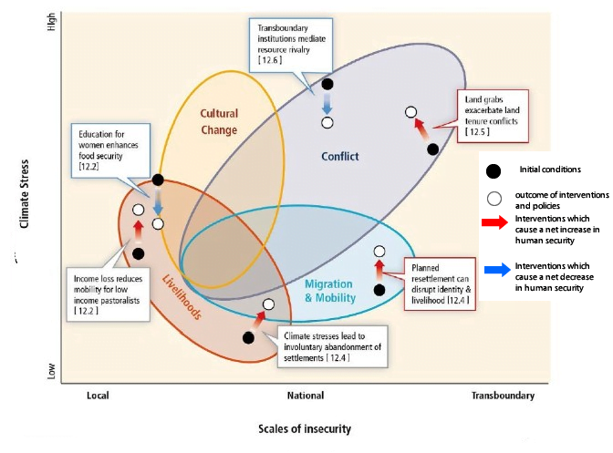
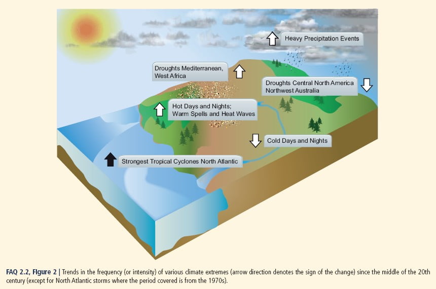
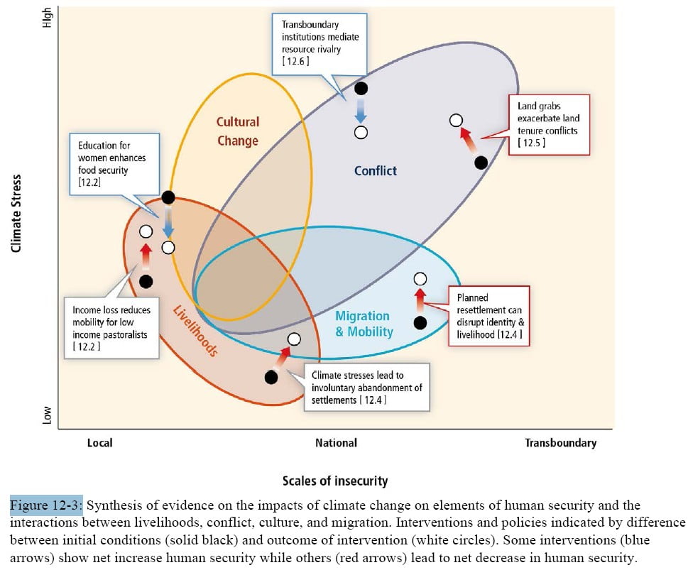
Human security will be progressively threatened as the climate changes. Human insecurity almost never has single causes, however climate change is an important factor through;

a) increasing migration that people would rather have avoided,

b) undermining livelihoods,

c) challenging the ability of states to provide the conditions necessary for human security,

d) compromising cultural values that are important for community and individual wellbeing.

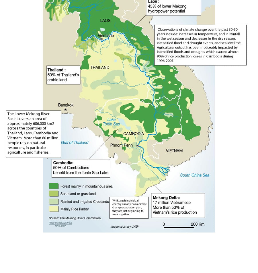
Migration and mobility are ways people adapt to climate variability in all regions of the world. In the past, major extreme weather events have led to significant population displacement, and changes in the incidence of extreme events will amplify the challenges and risks of such displacement. However, many vulnerable groups, particularly in rural and urban areas in low and middle-income countries, do not have the resources to be able to migrate to avoid the impacts of floods, storms and droughts. Migration may be undesirable, and can lead to changes in important cultural expressions and practices, and, in the absence of institutions to manage the settlement and integration of migrants in destination areas, can increase the risk of poverty, discrimination, violent conflict and inadequate provision of public services, public health and education.

Future challenges of climate change:

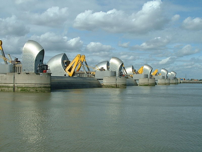
A) Physical impacts: Sea level rise, extreme events and hydrological disruptions, pose major challenges to vital transport, water, and energy infrastructure and can weaken states socially and economically.

B) Territorial impacts: For example those highly vulnerable to sea level rise.

C) Transboundary impacts: Changes in sea ice, shared water resources, and the migration of fish stocks, have the potential to increase rivalry among states.

D) Violent conflict can in turn undermine livelihoods, impel migration and weaken valued cultural expressions and practices.

E) Adaptation and mitigation strategies, such as those which develop large infrastructure or the resettle communities against their will to reduce exposure to climate change, carry risks of disrupted livelihoods, displaced populations, deterioration of valued cultural expressions and practices, and in some cases violent conflict.

In summary, climate change is one of many risks to the vital core of material well-being and culturally specific elements of human security that varies depending on location and circumstance.

On the basis of current evidence about the observed impacts of climate change on environmental conditions, climate change will be an increasingly important cause of human insecurity globally in the future. The greater the impact of climate change, the harder it is to adapt.

IPCC links

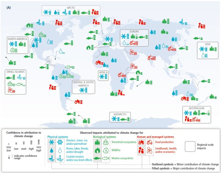
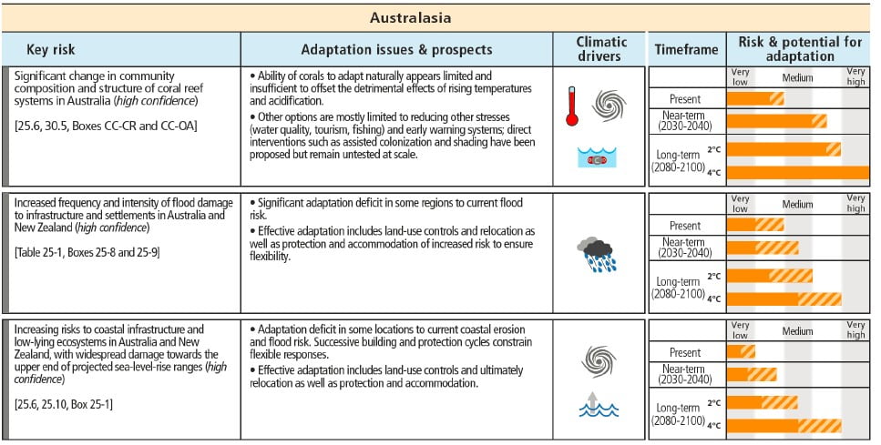
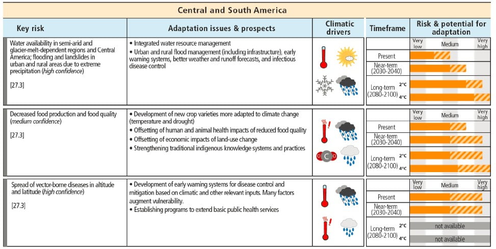
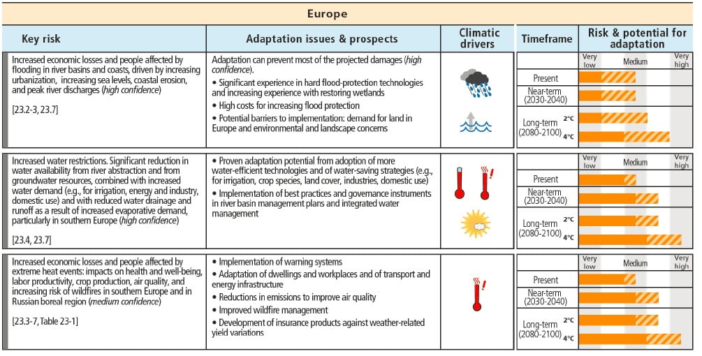
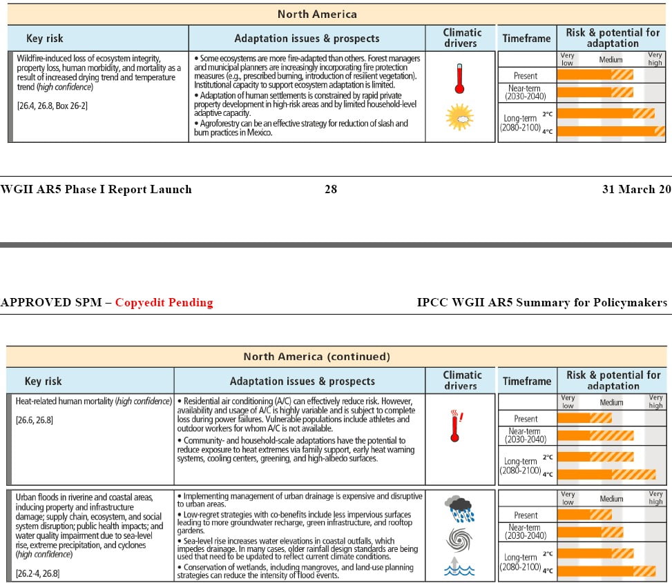
This is Figure 12.3 from the WGII report for the 2014 IPCC 5AR.

WGII FAQ 12.1: What are the principal threats to human security from climate change?

WGII FAQ 12.3: How many people could be displaced as a result of climate change?

WGII FAQ12.4: What role does migration play in adaptation to climate change, particularly in vulnerable regions?

WGII FAQ 12.5: Will climate change cause war between countries?

GLOSSARY

Aerosols A suspension of airborne solid or liquid particles, with a typical size between a few nanometres and 10 μm that reside in the atmosphere for at least several hours.

Anthropogenic Resulting from or produced by human activities.

Atlantic Meridional Overturning Circulation A major current in the Atlantic Ocean, characterized by a northward flow of warm, salty water in the upper layers of the Atlantic, and a southward flow of colder water in the deep Atlantic. It includes the North Atlantic Drift and the Gulf Stream.

Attribution The process of evaluating the relative contributions of multiple causal factors to a change or event with an assignment of statistical confidence

Climate The average weather, or more rigorously, the statistical description in terms of the mean and variability of relevant quantities over a period of time ranging from months to thousands or millions of years. The classical period for averaging these variables is 30 years, as defined by the World Meteorological Organization. The relevant quantities are most often surface variables such as temperature, precipitation and wind.

Climate Change A change in the state of the climate that can be identified (e.g. by using statistical tests) by changes in the mean and/or the variability of its properties, and that persists for an extended period, typically decades or longer. Climate change may be due to natural internal processes or external forcings such as modulations of the solar cycles, volcanic eruptions, and persistent anthropogenic changes in the composition of the atmosphere or in land use.

Climate Model A numerical representation of the climate system based on the physical, chemical and biological properties of its components, their interactions and feedback processes, and accounting for some of its known properties. Climate models are applied as a research tool to study and simulate the climate, and for operational purposes, including monthly, seasonal and interannual climate predictions.

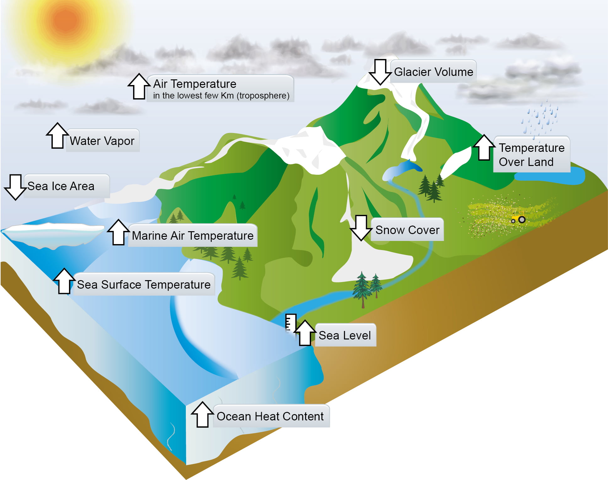
Cryosphere All regions on and beneath the surface of the Earth and ocean where water is in solid form, including sea ice, lake ice, river ice, snow cover, glaciers and ice sheets, and frozen ground (which includes permafrost).

Drought A period of abnormally dry weather long enough to cause a serious hydrological imbalance. Drought is a relative term; therefore any discussion in terms of precipitation deficit must refer to the particular precipitation-related activity that is under discussion.

Feedback An interaction in which a perturbation in one climate quantity causes a change in a second, and the change in the second quantity ultimately leads to an additional change in the first. A negative feedback is one in which the initial perturbation is weakened by the changes it causes; a positive feedback is one in which the initial perturbation is enhanced.

Forcings Forcing represents any external factor that influences global climate by heating or cooling the planet. Examples of forcings are volcanic eruptions, solar and orbital variations and anthropogenic (human) changes to the composition of the atmosphere.

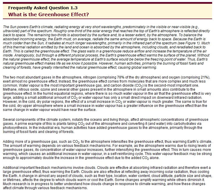
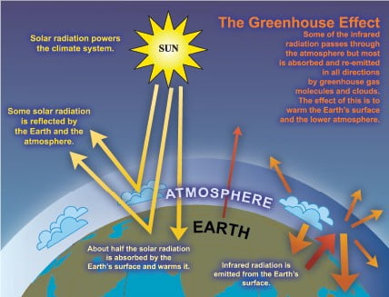
Greenhouse Gas Those gaseous constituents of the atmosphere, both natural and anthropogenic, that absorb and emit radiation at specific wavelengths within the spectrum of terrestrial radiation emitted by the Earth’s surface, the atmosphere itself, and by clouds.

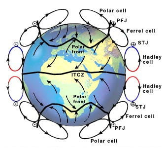
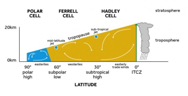
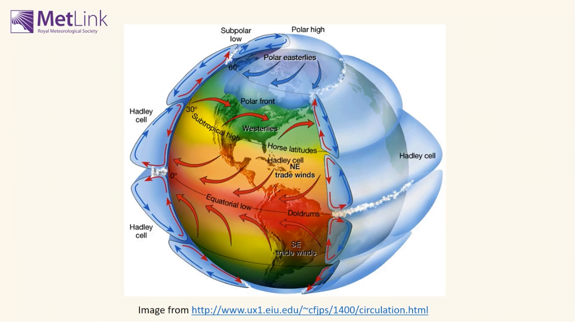
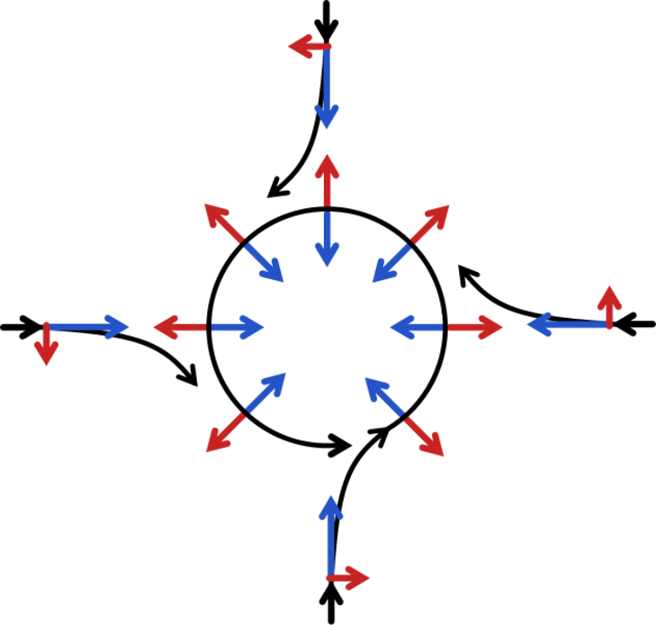
Hadley Cell A direct, thermally driven overturning cell in the atmosphere consisting of poleward flow in the upper troposphere, subsiding air into the subtropical anticyclones, return flow as part of the trade winds near the surface, and with rising air near the equator in the so-called Intertropical Convergence Zone.

Internal variability Variations in the mean state and other statistics (such as the occurrence of extremes) of the climate on all spatial and temporal scales beyond that of individual weather events, due to natural unforced processes within the climate system because, in a system of components with very different response times and complex dependencies, the components are never in equilibrium and are constantly varying. An example of internal variability is El Niño, a warming cycle in the Pacific Ocean which has a big impact on the global climate, resulting from the interaction between atmosphere and ocean in the tropical Pacific.

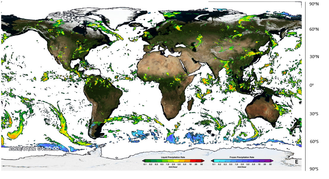
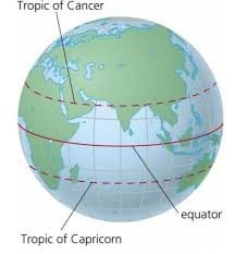
Inter-Tropical Convergence Zone The Inter-Tropical Convergence Zone is an equatorial zonal belt of low pressure, strong convection and heavy precipitation near the equator where the northeast trade winds meet the southeast trade winds. This band moves seasonally.

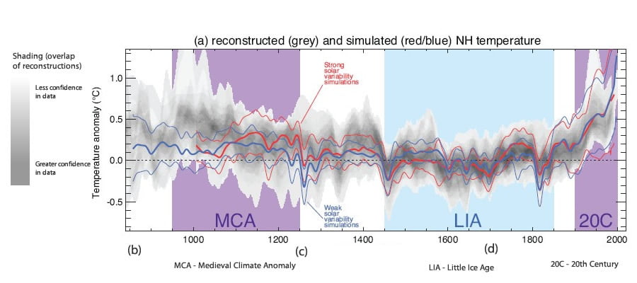
Paleoclimate Climate during periods prior to the development of measuring instruments, including historic and geologic time, for which only proxy climate records are available.

Pelagic Any water in a sea or lake that is neither close to the bottom nor near the shore.

Phenology The study of periodic plant and animal life cycle events and how these are influenced by seasonal and interannual variations in climate, as well as habitat factors.

Mitigation A human intervention to reduce the amount of climate change for example by reducing the sources or enhance the sinks of greenhouse gases.

Reconstruction Approach to reconstructing the past temporal and spatial characteristics of a climate variable from predictors. The predictors can be instrumental data if the reconstruction is used to infill missing data or proxy data if it is an indirect measure used to develop paleoclimate reconstructions.

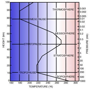
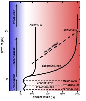
Stratosphere The highly stratified region of the atmosphere above the troposphere extending from about 10 km (ranging from 9 km at high latitudes to 16 km in the tropics on average) to about 50 km altitude.

Troposphere The lowest part of the atmosphere, from the surface to about 10 km in altitude at mid-latitudes (ranging from 9 km at high latitudes to 16 km in the tropics on average), where clouds and weather phenomena occur. In the troposphere, temperatures generally decrease with height.

Uncertainty A state of incomplete knowledge that can result from a lack of information or from disagreement about what is known or even knowable. It may have many types of sources, from imprecision in the data to ambiguously defined concepts or terminology, or uncertain projections of human behaviour.

UK National Curriculum Links

KS3 geography

  • Physical geography relating to: weather and climate, including the change in climate from the Ice Age to the present.
  • Understand how human and physical processes interact to influence, and change landscapes, environments and the climate; and how human activity relies on effective functioning of natural systems.

GCSE Geography

  • Changing weather and climate – The causes, consequences of and responses to extreme weather conditions and natural weather hazards, recognising their changing distribution in time and space and drawing on an understanding of the global circulation of the atmosphere. The spatial and temporal characteristics, of climatic change and evidence for different causes, including human activity, from the beginning of the Quaternary period (2.6 million years ago) to the present day.