Carbon is one of the building blocks of life. Humans, animals and plants are made up of organic compounds. We burn wood and fossil fuels to produce energy and power transport, inadvertently releasing the greenhouse gas, CO2 into the atmosphere.
We will look at a series of calculations that represent the carbon cycle and how CO2 production is related to energy. You will start to see the energy implications of various fuels and technologies and their CO2 footprint.
The associated information sheet will provide the data you need to answer the questions below.
How much CO2 is emitted by the following activities? (calculate them in kg of CO2)
Driving 100 miles?
(Using 13 litres of petrol or 10 litres diesel)
Using your LED TV for 5 hours a day during a week?
(A 50” LED TV uses 100 watts, to convert to kWh, multiply kW by number of hours)
Boiling water in the electric kettle for a family for a week?
(A kettle uses 1200 W and it takes 3 minutes to boil water and this is done 10 times a day – or does your household drink more hot drinks?)
Heating the water with natural gas for a week of daily 5 minute showers?
(Heating 30 litre of water to 40°C uses 1.1 kWh in the form of gas, where emissions from natural gas are 0.2 kg CO2/ kWh burned)
Charging mobile phones for the family for a week. With an average of two full charges a day.
(Typical phone charges at 0.015 kWh and takes 2 hours to charge fully)
Play station for 20 hours a week
(A Playstation 4 Pro uses 139 W)
2. How to quantify CO2 emissions in terms of volume and mass?
How many cubic metres of CO2 would 5000 kg CO2 occupy?
A factory states that it releases 10 tons C per year (as greenhouse gas emissions). How many m3 of CO2e is this?
If UK car emissions released 3 GtC in a year and all the CO2 remained in the atmosphere, by how much would the CO2 concentration increase?
Go to see last year´s UK Carbon emissions published by the government (Provisional GHG emissions). In 2019 it was 351.5 Mt CO2 Considering the UK population is 63 million and the world population is 8.3 billion, are our carbon emissions representative of global average emissions? ((World emissions in 2017 were 36 Bt)
What is today´s CO2 concentration at Mauna Loa (https://www.esrl.noaa.gov/gmd/ccgg/trends/)? How much has it increased since 1950? How much has it increased since the same month in 2018?
Why has CO2 not decreased in 2020 if CO2 emissions have dropped? Is there still last years and the decade before´s emissions in the air or are we still emitting more despite the drop in transport and industry in 2020?
3. Steps towards reaching carbon neutrality
Do you think the UK is on its way to becoming a low carbon economy? Why do you think some countries like Estonia are way behind the UK and countries like Sweden are way ahead?
The UK has a goal of reaching Carbon neutrality by 2050- do you think we are on our way to reaching that?
What percentage of our man-made CO2 emissions are absorbed by the oceans?
If a fully grown tree absorbs 22 kg of CO2 per year and an acre of forests 2.5 tons of Carbon, if we wanted to neutralize our country-wide annual emissions of 351.5Mt* CO2, how many more trees or acres of forest would we need?**
Carbon is one of the building blocks of life. Humans, animals and plants are made up of organic compounds. We burn wood and fossil fuels to produce energy and power transport, inadvertently releasing the greenhouse gas, CO2 into the atmosphere. Students will become more aware of the facts and figures that link the carbon cycle with CO2 emissions and the jargon that is used in the news and in global climate politics.
Chemistry curriculum links: AQA GCSE
3.2.1 Use of amount of substance in relation to masses of pure substances (Moles)
7.1 Carbon compounds as fuels and feedstock
9.2 Carbon dioxide and methane as greenhouse gases
9.2.4 The carbon footprint and its reduction
Chemistry in the activity
Calculating the energy from combustion of different fuels is related to the number of Carbon atoms these hydrocarbons contain. The amount of CO2 produced upon combustion is our way of measuring the Carbon footprint of energy sources. Electricity is generated from various forms of energy in each country´s electricity mix and the more renewables and the fewer inefficient coal power plants there are, the less CO2 is released per kWh electricity used. The UK is trying to go below 100 g of CO2 released per kWh by 2030 and is likely to achieve this before that date.
In the associated worksheet the students will carry out calculations based on a range of information they will find in the corresponding information sheet. They will become familiar with conversions between tons of Carbon and tons of CO2, the volume of CO2 and other factors they may hear in the news or that relate to their personal, a country´s or organisation´s carbon emissions.
They will go to websites that provide current global CO2 levels and a breakdown of the UK´s electricity supply, with the corresponding kg of CO2 this will emit per unit electricity used. Questions 1&2 use numeracy skills to evaluate and compare different forms of energy and different technologies.
Question 3 is best used as a classroom discussion and covers carbon neutrality, achieving the UK´s Carbon neutrality goals and calculate how many trees they would have to plant to neutralise this year´s CO2 emissions.
1. Which fuels or activities produce more CO2?
QUESTIONS
Which of these activities produces more CO2 emissions? (calculate them in kg of CO2)
Driving 100 miles?
(Using 13 litres of petrol or 10 litres of diesel)
Petrol = 2.3 x 13, Diesel = 2.7 x 10 = 29.9 kg CO2 for petrol and 27 kg for diesel
Using your LED TV for 5 hours a day during a week?
(A 50” LED TV uses 100 watts, to convert to kWh, multiply kW by number of hours)
5 x 7 hours at 100 watts = 3.5 kWh = 3.5 kg CO2
Boiling water in the electric kettle for a family for a week?
(A kettle uses 1200 W and it takes 3 minutes to boil water and this is done 10 times a day – or does your family drink more tea?)
1200 x 10 x 3 x 7 = 210 minutes (3.5 hours) or 4.2 kWh x 0.283 = 1.19 kg CO2
Heating the water with natural gas for a week of daily 5 minute showers?
(Heating 30 litre of water to 40°C uses 1.1 kWh in the form of gas, where emissions from natural gas are 0.2 kg CO2/ kWh burned)
Heating the water for a week uses 7.7 kWh so 0.2 x 7.7 is 1.54 kg CO2
Mobile phone usage for the family in a week. Assume the family does an average of two full charges a day.
(Typical phone charges at 0.015 kWh and takes 2 hours to charge fully)
4 x 7 x 0.005 = 0.014 kWh x 0.283 = 0.396 kg CO2
Play station for 20 hours a week
(A Playstation 4 Pro uses 139 W)
139 x 20 = 2.4 kWh = 7.87 kg CO2
2. How to quantify CO2 emissions in terms of volume and mass?
QUESTIONS
How many cubic metres of CO2 would 5000 kg CO2 occupy? 2500 m3
A factory states that it releases 10 tons C per year (for its greenhouse gas emissions). How many m3 of CO2e is this? 10,000 kg x 44/12 = 36,667 kg CO2, so ½ x this is 18,333 m3
If UK car emissions released 3 GtC in a year and all the CO2 remained in the atmosphere, by how much would the CO2 concentration increase?
0.47 x 3 = 1.41 ppmv
Go to see last year´s UK Carbon emissions published by the government (Provisional GHG emissions). In 2019 it was 351.5 Mt CO2 Considering the UK population is 63 million and world population is 8.3 billion, are our carbon emissions representative of global average emissions? ((World emissions in 2017 were 36 Bt)
63m/8.3b =0.81 % of population and CO2 emissions are 351.5Mt/36000Mt = 0.98 %, so the population of the UK creates more CO2 than their population dictates, we produce 0.98/0.81 =1.21 times more CO2 than the average world population
What is today´s CO2 concentration at Mauna Loa (https://www.esrl.noaa.gov/gmd/ccgg/trends/)? How much has it increased since 1950? How much has it increased since the same month in 2018?
(figures for 2020) 500 ppm; increase of 100 ppm between 1950 and 2020 (in 70 years), that is a 0.7 ppm average increase; it has increased 4 ppm since 2018 (in 2 years), 2 ppm increase per year. The rate of increase of CO2 concentration has increased since the 1950s.
Why has CO2 concentration not decreased in 2020 if CO2 emissions have dropped?
The lifetime of CO2 means that it stays around in the atmosphere for many years and you will not see a decrease in the CO2 from the year that you stop releasing it, it will gradually level off, that is why we need to reach our CO2 emission peak as early as possible, to see the results a few years later.
3. Steps towards reaching carbon neutrality
QUESTIONS to discuss as a class
Do you think the UK is on its way to becoming a low carbon economy? Why do you think some countries like Estonia are way behind the UK and countries like Sweden are way ahead? (http://www.globalcarbonatlas.org/en/CO2-emissions is a useful information source)
Estonia still burns a lot of coal, hence its high CO2 emissions. Sweden has 80 % of its electricity from nuclear and renewables
The UK has a goal of reaching Carbon neutrality by 2050- do you think we are on our way to reaching that?
What percentage of our anthropogenic (human) CO2 emissions are absorbed by the oceans?
31 %
If a fully grown tree absorbs 22 kg of CO2 per year and an acre of forest, 2.5 tons of Carbon, if we wanted to neutralize our country-wide annual emissions of 351.5Mt* CO2, how many more trees or acres of forest would we need?**
351500/2.5 = 140600 acres. There are 60 million acres in the UK, so actually, only adding 0.234 % of the land as forests would do this!
Carbon is one of the building blocks of life. Humans, animals and plants are made up of organic compounds. We burn wood and fossil fuels to produce energy and power transport, inadvertently releasing the greenhouse gas, CO2 into the atmosphere.
1. Which fuels or activities produce more energy or CO2?
What are fossil fuels made up of? Hydrocarbons with varying amounts of Carbon:
Coal contains large complex hydrocarbon molecules (with C:H:O ratios of ~85C:5H:10O)
Diesel is made up of alkanes containing 12 or more carbon atoms. (e.g. C13H28)
Petrol contains alkanes and cyclo-alkanes with between 5 and 12 Carbon atoms (with an average composition of C8H12 (octane))
The mass of one mole of pure Carbon is 12 g and the mass of one mole of CO2 is 12 + (2×16) = 44 g (to convert from CO2e to C multiply by 12/44)
What are the combustion reactions and how much energy and CO2 do they produce?
1 kg of petrol burned yields about 47 MJ of energy (1litre, 34.2MJ)
1 kg of diesel burned yields about 46 MJ of energy (1litre, 38.6MJ) (diesel is denser than petrol and has more energy per litre)
1 kg of coal burned yields about 30 MJ of energy
1 kg of wood burned yields about 19 MJ of energy
1 kg of coal (containing 0.78 kg Carbon) will produce 2.4 kg of CO2
1 litre of petrol (containing 0.63 kg of carbon) will produce 2.3 kg of CO2
1 litre of diesel (containing 0.72 kg of carbon) will produce 2.7 kg of CO2
The most up-to-date information on the make-up of the UK electricity grid (which is a mix of sources) can be found at RENSmart and the value in February 2021 was that 1 kWh produces 0.23314 kg CO2. (kWh are calculated by multiplying kW by the number of hours). If you live in another country you could compare its CO2 emissions per kWh electricity factor. Here is a good comparison site for many countries but with older data.
2. How to quantify CO2 emissions in terms of volume and mass?
Volume and mass of CO2
You will often hear about kg of CO2 emitted, relating to the energy usage of different forms of transport, of a household, of a company, of a particular industry (like the cement industry) or of a country or a person.
From what we know about the combustion processes, their efficiency and our energy needs, we can use emission factors to calculate carbon footprints. We also know that a mole of any gas occupies 22.4 dm3 at ambient temperature. So we can express the emissions as a volume of CO2. If we know how much of a gas is emitted and what the original concentration of that gas was in the atmosphere, we can see whether the emissions will change the concentration.
1 kg pure CO2 occupies a volume of half a cubic metre (500 dm3 (or litres))
CO2 emissions are often stated in GtC (109 tonnes (or Gigatonnes) of Carbon)
Concentrations of CO2 in the atmosphere are expressed in parts per million by volume (ppmv). 1 ppmv takes up 0.0001% of the volume of the atmosphere. Check out the Mauna Loa CO2 measurement station in Hawai for today´s level.
A release of CO2containing 1 GtC would increase the atmospheric CO2 concentration by 0.47 ppmv if all the CO2 remained in the atmosphere, BUT carbon sinks nearly balance out the sources
There was a CO2 increase of 2.5 ± 0.1 ppmv between 2017 and 2018
The lifetime of CO2 is 5 to 100 years
Don’t forget:
The mass of one mole of pure Carbon is 12 g and the mass of one mole of CO2 is 12 + (2×16) = 44 g (to convert from CO2eq to C multiply by 12/44)
Effects of the Covid-19 on the economy and thus CO2 emissions
Between 2019 and 2020 global CO2 emissions decreased due to the COVID-19 Pandemic (in the region of 4 Gt CO2 and the CO2 emissions fell by 7 % in 2020, the largest ever decrease since the Second World War!)
A Carbon brief article suggests that in 2020 we reduced the annual increase in CO2 concentrations by 0.32ppmv, putting it at 2.48ppm.
Note the difference between emissions of CO2 and actual concentrations. The CO2 already in the atmosphere from previous year´s emissions (it lasts up to one hundred years).
3. Steps towards carbon neutrality
This Figure shows the latest (calculated every 3 months) fuel source mix for the UK electricity supply. Go to: OFGEM. Note the elimination of coal and the increase in wind and solar energy.
The UK electricity supply now has well over 20 % from renewables. The UK is trying to get to below 100 g CO2/ kWh by 2030 and we might achieve 5 % renewables by 2025. In late 2019 the electricity from British windfarms, solar panels and renewable biomass plants surpassed fossil fuels for the first time since the UK’s first power plant fired up in 1882.
We saw in section 1 that at RENSmart you can get the latest value for how many kg CO2 are produced per kWh of electricity. Let´s compare other countries from the table at the bottom of this website. Sweden currently has an emission of 0.013 kg CO2/ kWh (21 times lower CO2 emissions per kWh!). In Sweden 80 % of electricity comes from nuclear and renewables (with 66 % from renewables). By the way, renewables do have an embedded energy (of up to 50 g CO2/ kWh).
And look what these natural Carbon Sinks can do:
Between 1994 and 2007, the oceans absorbed 34 Gt CO2 (31 % of what humans put into the atmosphere during that time)
One acre of new forest can sequester about 2.5 tons of carbon annually. Young trees absorb CO2 at a rate of 6 kg per tree each year and after 10 years they absorb 22 kg of CO2 per year. At that rate, they release enough oxygen back into the atmosphere to support two human beings.
Carbon, water, weather and climate a PowerPoint presentation focussing on recent changes to the carbon and water cycles, and how the two cycles interact.
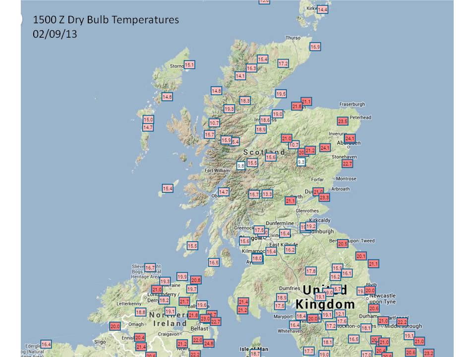
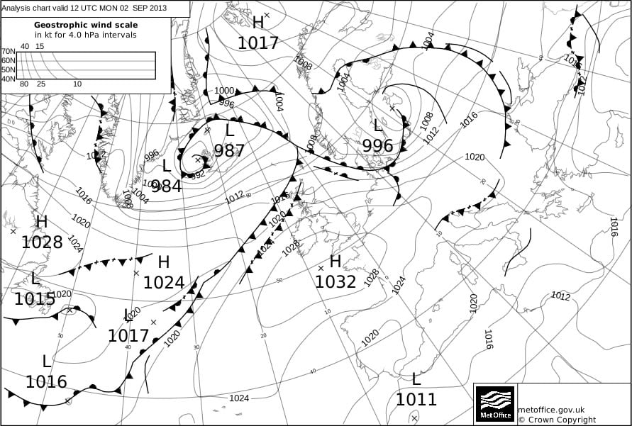
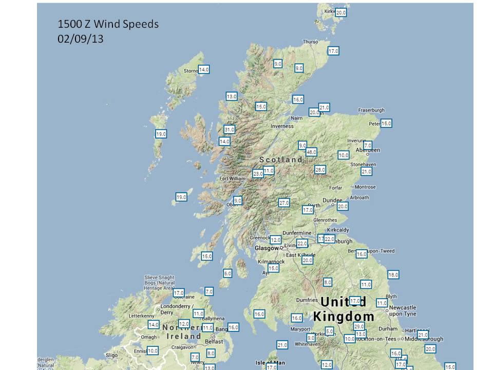
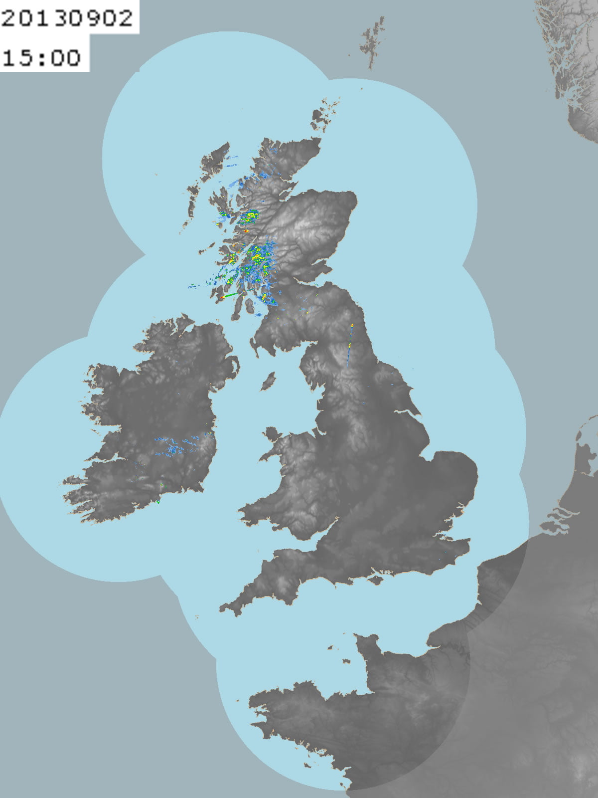
Depression based exercise where students draw contours of temperature, pressure and precipitation to work out what the system looks like: Student worksheets and notes for teachers. Simpler versions of the same exercise can be found on the KS3/4 web pages.
This news item from NASA relates to this animation, as does this Nature Communication from October 2020.
Suggested learning activities:
Data and GIS exercise for A Level students
Explore leaf area, evapotranspiration and temperature data using various statistical techniques to explore the relationship between deforestation and weather on this resource on the RGS website.
Activity 1: Ask students to write a voiceover for the film, demonstrating their understanding of the concepts involved.
Activity 2: Complete this sentence based on the film: When rainforests are deforested, places downwind are left with more/ less/ the same amount of rainfall and greater/ less/ the same amount of flood risk.
Activity 3: Look at www.globalforestwatch.org/map and identify a Tropical region which has experienced deforestation in the last decade. Look at earth.nullschool.net. What is the prevailing wind direction in that region? Using www.google.com/maps, write a paragraph explaining how you think the water cycle has been affected by deforestation for a place downwind from the rainforest region you identified.
Activity 5: Having watched the animation, read these articles from Nature and NASA (noting that this predates the Nature article), NASA (2019), Geography Review (p22 – 25) and Carbon Brief. Summarise the impact of tropical deforestation on the carbon and water cycles.
Carbon (chemical element C) is one of the most abundant elements in the universe.
All known life forms are carbon-based and it amounts to about 18% of a human body.
Carbon dioxide (CO2) and methane (CH4) make up about 0.04% of our atmosphere by volume.
However, alongside water vapour, nitrous oxide and ozone (collectively called greenhouse gases) they help to keep our planet warm.
In fact, without these gases, the Earth’s surface would be about 18 °C below zero – far too cold for nearly all life to survive. Greenhouse gases occur naturally, but human activities have directly increased the amount of carbon dioxide, methane and some other gases in our atmosphere. There is overwhelming evidence that this has enhanced the natural greenhouse effect, contributing to the warming we have seen over the last century or so. For more information on this visit our in depth climate section
When studying our climate, scientists draw their evidence from many sources. It is important that they look at all the processes that influence our climate, and one of the most important is the carbon cycle.
Web page reproduced with the kind permission of the Met Office
Questions to consider:Name one positive and one negative feedback to climate change from the ocean’s biological pump. What is the difference between the fast domain and the slow domain within the global carbon cycle? How has the transfer of carbon changed between these two domains post industrialisation?
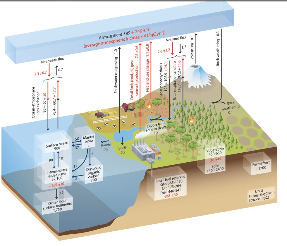
WG1 Chapter 6, figure 1. The numbers represent carbon reservoirs in Petagrams of Carbon (PgC; 1015gC) and the annual exchanges in PgC/year. The black numbers and arrows show the pre-Industrial reservoirs and fluxes. The red numbers and arrows show the additional fluxes caused by human activities averaged over 2000-2009, which include emissions due to the burning of fossil fuels, cement production and land use change (in total about 9 PgC/year). Some of this additional anthropogenic carbon is taken up by the land and the ocean (about 5 PgC/year) while the remainder is left in the atmosphere (4 PgC/year), explaining the rising atmospheric concentrations of CO2. The red numbers in the reservoirs show the cumulative changes in anthropogenic carbon from 1750-2011; a positive change indicates that the reservoir has gained carbon.
Summary:
The global carbon cycle can be viewed as a series of reservoirs of carbon in the Earth System, which are connected by exchange fluxes of carbon. An exchange flux is the amount of carbon which moves between reservoirs each year.
Before human activities such as land use changes and industrial processes had a significant impact, the global carbon cycle was roughly balanced.
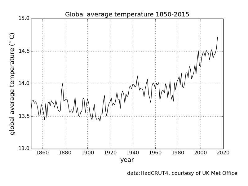
CO2 increased by over 40% from around 280 ppm in 1750 to 400 ppm in 2015.
Higher atmospheric CO2 concentrations, and associated climate impacts of present emissions, will persist for hundreds of years into the future.
Carbon, water, weather and climate a PowerPoint presentation focussing on recent changes to the carbon and water cycles, and how the two cycles interact.
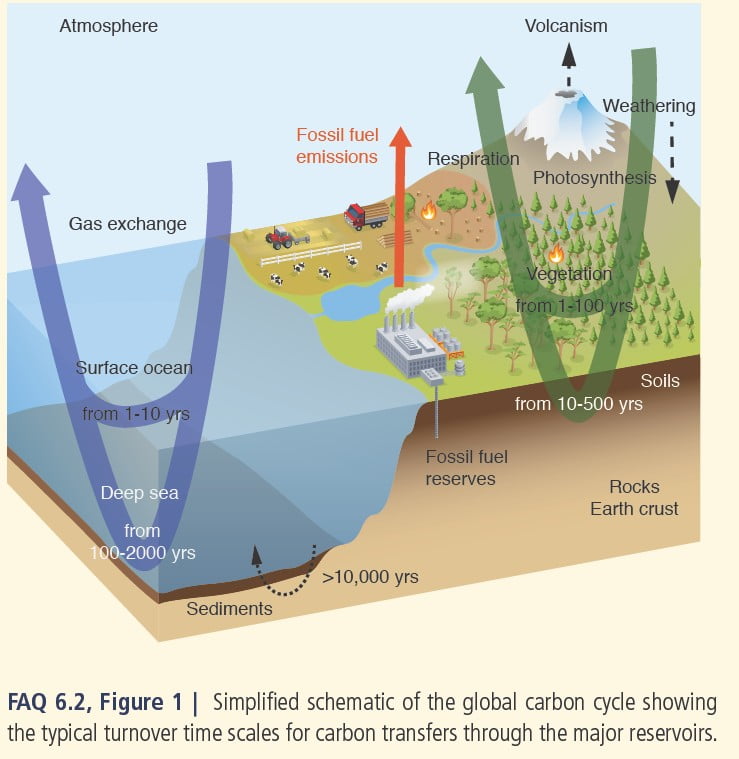
How fast is the carbon cycle? There are two domains in the global carbon cycle, fast and slow. The fast domain has large exchange fluxes and relatively ‘rapid’ reservoir turnovers. This includes carbon on land in vegetation, soils, peat and freshwater and in the atmosphere, ocean and surface ocean sediments. Reservoir turnover times (a measure of how long the carbon stays in the reservoir) range from a few years for the atmosphere to decades to millennia for the major carbon reservoirs of the land vegetation and soil and the various domains in the ocean.
The slow domain consists of the huge carbon stores in rocks and sediments which exchange carbon with the fast domain through volcanic emissions of CO2, erosion and sediment formation on the sea floor. Reservoir turnover times of the slow domain are 10,000 years or longer.
Before the Industrial Era, the fast domain was close to a steady state. Data from ice cores show little change in the atmospheric CO2 levels over millennia despite changes in land use and small emissions from humans. By contrast, since the beginning of the Industrial Era (around 1750), fossil fuel extraction and its combustion have resulted in the transfer of a significant amount of fossil carbon from the slow domain into the fast domain, causing a major change to the carbon cycle.
Some reservoirs of carbon: In the atmosphere, CO2 is the dominant carbon containing trace gas with a mass of 828 PgC (Petagrams of Carbon or x1015gC). Additional trace gases include methane (CH4, currently about 3.7 PgC) and carbon monoxide (CO, around 0.2 PgC), with still smaller amounts of hydrocarbons, black carbon aerosols and other organic compounds.
The terrestrial biosphere reservoir contains carbon in organic compounds in vegetation (living biomass) (450 to 650 PgC) and in dead organic matter in litter and soils (1500 to 2400 PgC). There is an additional amount of old soil carbon in wetland soils (300 to 700 PgC) and in permafrost (1700 PgC).
Some fluxes of carbon:
CO2 is removed from the atmosphere by plant photosynthesis (123±8 PgC/ year). Carbon fixed into plants is then cycled through plant tissues, litter and soil carbon and can be released back into the atmosphere by plant, microbial and animal respiration and other processes (e.g. forest fires) on a very wide range of time scales (seconds to millennia).
A significant amount of terrestrial carbon (1.7 PgC/year) is transported from soils to rivers. A fraction of this carbon is released as CO2 by rivers and lakes to the atmosphere, a fraction is buried in freshwater organic sediments and the remaining amount (~0.9 PgC/ year) is delivered by rivers to the coastal ocean. Atmospheric CO2 is exchanged with the surface ocean through gas exchange.
Carbon is transported within the ocean by three mechanisms;
(1) the ‘solubility pump’ (see glossary), (2) the ‘biological pump’ (see case study), (3) the ‘marine carbonate pump’ which is caused by marine organisms forming shells in the surface ocean. These sink, are buried in the sediments and eventually form sedimentary rocks (such as limestone or chalk).
Changes to the carbon cycle
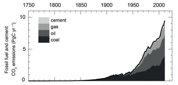
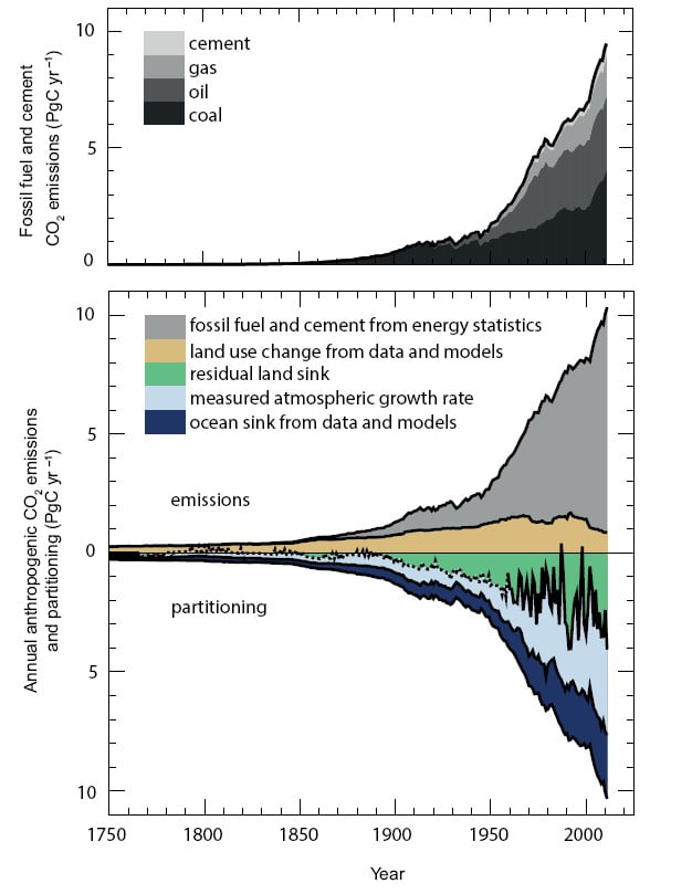
WG1 Technical Summary Figure 4. Annual global anthropogenic CO2 emissions (PgC/ year) from 1750 to 2011
Anthropogenic CO2 emissions to the atmosphere were 555 ± 85 PgC between 1750 and 2011. Of this, fossil fuel combustion and cement production contributed 375 ± 30 PgC and land use change (including deforestation, afforestation (planting new forest) and reforestation) contributed 180 ± 80 PgC. In 2002–2011, average fossil fuel and cement manufacturing emissions were 7.6 to 9.0 PgC/ year, with an average increase of 3.2%/ year compared with 1.0%/ year during the 1990s. In 2011, fossil fuel emissions were in the range of 8.7 to 10.3 PgC.
Emissions due to land use changes (primarily tropical deforestation) between 2002 and 2011 are estimated to range between 0.1 to 1.7 PgC/year. This includes emissions from deforestation of around 3 PgC/ year compensated by an uptake of around 2 PgC/year by forest regrowth (mainly on abandoned agricultural land).
The IPCC concluded that the increase in CO2 emissions from both fossil fuel burning and land use change are the dominant cause of the observed increase in atmospheric CO2 concentration.
Globally, the combined natural land and ocean sinks of CO2 kept up with the atmospheric rate of increase, removing 55% of the total anthropogenic emissions every year on average during 1958–2011. The ocean reservoir stored 155 ± 30 PgC. Vegetation biomass and soils stored 160 ± 90 PgC.
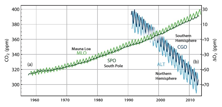
WG1 chapter 6, figure 3 Concentrations of carbon dioxide and oxygen in the atmosphere Atmospheric concentration of a) carbon dioxide in parts per million by volume from Mauna Loa (MLO, light green) and the South Pole (SPO, dark green) and of b) changes in the atmospheric concentration of O2 from the northern hemisphere (ALT, light blue) and the southern hemisphere (CGO, dark blue) relative to a standard value.
Carbon Dioxide concentrations in the atmosphere increased by over 40% from 278 ppm in 1750 to 400 ppm in 2015.
Most of the fossil fuel CO2 emissions take place in the industrialised countries north of the equator. Consistent with this, the annual average atmospheric CO2 measurement stations in the Northern Hemisphere (NH) record slightly higher CO2 concentrations than stations in the Southern Hemisphere (SH). As the difference in fossil fuel combustion between the hemispheres has increased, so has the difference in concentration between measuring stations at the South Pole and Mauna Loa (Hawaii, NH).
The atmospheric CO2 concentration increased by around 20 ppm during 2002–2011. This decadal rate of increase is higher than during any previous decade since direct atmospheric concentration measurements began in 1958.
Because CO2 uptake by photosynthesis occurs only during the growing season, whereas CO2 release by respiration occurs nearly year-round, both the Mauna Loa and South Pole concentrations show an annual cycle, with more CO2 in the atmosphere in winter. However, as there is far more land mass and therefore vegetation in the Northern Hemisphere, the annual cycle is more pronounced at Mauna Loa.
Past changes in atmospheric greenhouse gas concentrations can be determined with very high confidence from polar ice cores. During the 800,000 years prior to 1750, atmospheric CO2 varied from 180 ppm during glacial (cold) up to 300 ppm during interglacial (warm) periods. Present-day (2011) concentrations of atmospheric carbon dioxide far exceed this range. The current rate of CO2 rise in atmospheric concentrations is unprecedented with respect to the highest resolution ice core records which cover the last 22,000 years.
What is the relationship between the Carbon Cycle and Oxygen?
Atmospheric oxygen is tightly coupled with the global carbon cycle. The burning of fossil fuels removes oxygen from the atmosphere. As a consequence of the burning of fossil fuels, atmospheric O2 levels have been observed to decrease slowly but steadily over the last 20 years. Compared to the atmospheric oxygen content of about 21% this decrease is very small and has no impact on health; however, it provides independent evidence that the rise in CO2 must be due to an oxidation process, that is, fossil fuel combustion and/or organic carbon oxidation, and is not caused by volcanic emissions or a warming ocean releasing carbon dioxide (CO2 is less soluble in warm water than cold).
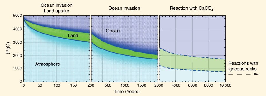
FAQ 6.2, Figure 2 illustrates the decay of a large excess amount of CO2 (5000 PgC, or about 10 times the cumulative CO2 emitted so far since the beginning of the industrial Era) emitted into the atmosphere, and how it is redistributed among land and the ocean over time. During the first 200 years, the ocean and land take up similar amounts of carbon. On longer time scales, the ocean uptake dominates mainly because of its larger reservoir size (~38,000 PgC) as compared to land (~4000 PgC) and atmosphere (589 PgC prior to the Industrial Era). Because of ocean chemistry the size of the initial input is important: higher emissions imply that a larger fraction of CO2 will remain in the atmosphere. After 2000 years, the atmosphere will still contain between 15% and 40% of those initial CO2 emissions. A further reduction by carbonate sediment dissolution, and reactions with igneous rocks, such as silicate weathering and sediment burial, will take anything from tens to hundreds of thousands of years, or even longer.
What Happens to Carbon Dioxide After It Is Emitted into the Atmosphere?
(WG1 FAQ6.2) Carbon dioxide (CO2), after it is emitted into the atmosphere, is firstly rapidly distributed between atmosphere, the upper ocean and vegetation. Subsequently, the carbon continues to be moved between the different reservoirs of the global carbon cycle, such as soils, the deeper ocean and rocks. Some of these exchanges occur very slowly. Depending on the amount of CO2 released, between 15% and 40% will remain in the atmosphere for up to 2000 years, after which a new balance is established between the atmosphere, the land biosphere and the ocean. Geological processes will take anywhere from tens to hundreds of thousands of years—perhaps longer—to redistribute the carbon further among the geological reservoirs. Higher atmospheric CO2 concentrations, and associated climate impacts of present emissions, will, therefore, persist for a very long time into the future. CO2 is a largely non-reactive gas, which is rapidly mixed throughout the entire troposphere in less than a year. Unlike reactive chemical compounds in the atmosphere that are removed and broken down by sink processes, such as methane, carbon is instead redistributed among the different reservoirs of the global carbon cycle and ultimately recycled back to the atmosphere on a multitude of time scales. Figure 1 shows a simplified diagram of the global carbon cycle. The open arrows indicate typical timeframes for carbon atoms to be transferred through the different reservoirs.
Before the Industrial Era, the global carbon cycle was roughly balanced. This can be inferred from ice core measurements, which show a near constant atmospheric concentration of CO2 over the last several thousand years prior to the Industrial Era. Anthropogenic emissions of carbon dioxide into the atmosphere, however, have disturbed that equilibrium. As global CO2 concentrations rise, the exchange processes between CO2 and the surface-ocean and vegetation are altered, as are subsequent exchanges within and among the carbon reservoirs on land, in the ocean and eventually, the Earth crust. In this way, the added carbon is redistributed by the global carbon cycle, until the exchanges of carbon between the different carbon reservoirs have reached a new, approximate balance. Over the ocean, CO2 molecules pass through the air-sea interface by gas exchange. In seawater, CO2 interacts with water molecules to form carbonic acid, which reacts very quickly with the large reservoir of dissolved inorganic carbon—bicarbonate and carbonate ions—in the ocean. Currents and the formation of sinking dense waters transport the carbon between the surface and deeper layers of the ocean. The marine biota also redistribute carbon: marine organisms grow organic tissue and calcareous shells in surface waters, which, after their death, sink to deeper waters, where they are returned to the dissolved inorganic carbon reservoir by dissolution and microbial decomposition. A small fraction reaches the sea floor, and is incorporated into the sediments.
The extra carbon from anthropogenic emissions has the effect of increasing the atmospheric partial pressure of CO2, which in turn increases the air-to-sea exchange of CO2 molecules. In the surface ocean, the carbonate chemistry quickly accommodates that extra CO2. As a result, shallow surface ocean waters reach balance with the atmosphere within 1 or 2 years. Movement of the carbon from the surface into the middle depths and deeper waters takes longer—between decades and many centuries. On still longer time scales, acidification by the invading CO2 dissolves carbonate sediments on the sea floor, which further enhances ocean uptake. However, current understanding suggests that, unless substantial ocean circulation changes occur, plankton growth remains roughly unchanged because it is limited mostly by environmental factors, such as nutrients and light, and not by the availability of inorganic carbon it does not contribute significantly to the ocean uptake of anthropogenic CO2.
Decay of a CO2 excess amount of 5000 PgC emitted at time zero into the atmosphere, and its subsequent redistribution into land and ocean as a function of time, computed by coupled carbon-cycle climate models. The sizes of the colour bands indicate the carbon uptake by the respective reservoir. The first two panels show the multi-model mean from a model intercomparison project. The last panel shows the longer term redistribution including ocean dissolution of carbonaceous sediments as computed with an Earth System Model of Intermediate Complexity.
On land, vegetation absorbs CO2 by photosynthesis and converts it into organic matter. A fraction of this carbon is immediately returned to the atmosphere as CO2 by plant respiration. Plants use the remainder for growth. Dead plant material is incorporated into soils, eventually to be decomposed by microorganisms and then respired back into the atmosphere as CO2. In addition, carbon in vegetation and soils is also converted back into CO2 by fires, insects, herbivores, as well as by harvest of plants and subsequent consumption by livestock or humans. Some organic carbon is furthermore carried into the ocean by streams and rivers.
An increase in atmospheric CO2 stimulates photosynthesis, and thus carbon uptake. In addition, elevated CO2 concentrations help plants in dry areas to use ground water more efficiently. This in turn increases the biomass in vegetation and soils and so fosters a carbon sink on land. The magnitude of this sink, however, also depends critically on other factors, such as water and nutrient availability.
Coupled carbon-cycle climate models indicate that less carbon is taken up by the ocean and land as the climate warms constituting a positive climate feedback. Many different factors contribute to this effect: warmer seawater, for instance, has a lower CO2 solubility, so altered chemical carbon reactions result in less oceanic uptake of excess atmospheric CO2. On land, higher temperatures foster longer seasonal growth periods in temperate and higher latitudes, but also faster respiration of soil carbon.
The time it takes to reach a new carbon distribution balance depends on the transfer times of carbon through the different reservoirs, and takes place over a multitude of time scales. Carbon is first exchanged among the ‘fast’ carbon reservoirs, such as the atmosphere, surface ocean, land vegetation and soils, over time scales up to a few thousand years. Over longer time scales, very slow secondary geological processes—dissolution of carbonate sediments and sediment burial into the Earth’s crust—become important.
How Does Anthropogenic Ocean Acidification Relate to Climate Change?
WG1 FAQ3.3 Both anthropogenic climate change and anthropogenic ocean acidification are caused by increasing carbon dioxide concentrations in the atmosphere. Rising levels of carbon dioxide (CO2), along with other greenhouse gases, indirectly alter the climate system by trapping heat as it is reflected back from the Earth’s surface. Anthropogenic ocean acidification is a direct consequence of rising CO2 concentrations as seawater currently absorbs about 30% of the anthropogenic CO2 from the atmosphere.
Ocean acidification refers to a reduction in pH over an extended period, typically decades or longer, caused primarily by the uptake of CO2 from the atmosphere. pH is a dimensionless measure of acidity. Ocean acidification describes the direction of pH change rather than the end point; that is, ocean pH is decreasing (the oceans are becoming less alkaline) but the oceans are not expected to become acidic (pH < 7). Ocean acidification can also be caused by other chemical additions or subtractions from the oceans that are natural (e.g., increased volcanic activity, methane hydrate releases, long-term changes in net respiration) or human-induced (e.g., release of nitrogen and sulphur compounds into the atmosphere). Anthropogenic ocean acidification refers to the component of pH reduction that is caused by human activity.
Since about 1750, the release of CO2 from industrial and agricultural activities has resulted in global average atmospheric CO2 concentrations that have increased from 278 to 390.5ppm in 2011. The atmospheric concentration of CO2 is now higher than experienced on the Earth for at least the last 800,000 years and is expected to continue to rise because of our dependence on fossil fuels for energy. To date, the oceans have absorbed approximately 155 ± 30 PgC from the atmosphere, which corresponds to roughly one-fourth of the total amount of CO2 emitted (555 ± 85 PgC) by human activities since preindustrial times. This natural process of absorption has significantly reduced the greenhouse gas levels in the atmosphere and minimized some of the impacts of global warming. However, the ocean’s uptake of CO2 is having a significant impact on the chemistry of seawater. The average pH of ocean surface waters has already fallen by about 0.1 units, from about 8.2 to 8.1 since the beginning of the Industrial Revolution. Estimates of projected future atmospheric and oceanic CO2 concentrations indicate that, by the end of this century, the average surface ocean pH could be 0.2 to 0.4 lower than it is today. The pH scale is logarithmic, so a change of 1 unit corresponds to a 10-fold change in hydrogen ion concentration.
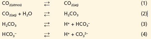
When atmospheric CO2 exchanges across the air–sea interface it reacts with seawater through a series of four chemical reactions that increase the concentrations of the carbon species: dissolved carbon dioxide (CO2(aq)), carbonic acid (H2CO3) and bicarbonate (HCO3–)
Hydrogen ions (H+) are produced by these reactions. This increase in the ocean’s hydrogen ion concentration corresponds to a reduction in pH, or an increase in acidity. Under normal seawater conditions, more than 99.99% of the hydrogen ions that are produced will combine with carbonate ion (CO32–) to produce additional HCO3–. Thus, the addition of anthropogenic CO2 into the oceans lowers the pH and consumes carbonate ion. These reactions are fully reversible and the basic thermodynamics of these reactions in seawater are well known, such that at a pH of approximately 8.1 approximately 90% the carbon is in the form of bicarbonate ion, 9% in the form of carbonate ion, and only about 1% of the carbon is in the form of dissolved CO2. Results from laboratory, field, and modelling studies, as well as evidence from the geological record, clearly indicate that marine ecosystems are highly susceptible to the increases in oceanic CO2 and the corresponding decreases in pH and carbonate ion.
Climate change and anthropogenic ocean acidification do not act independently. Although the CO2 that is taken up by the ocean does not contribute to greenhouse warming, ocean warming reduces the solubility of carbon dioxide in seawater; and thus reduces the amount of CO2 the oceans can absorb from the atmosphere. For example, under doubled preindustrial CO2 concentrations and a 2°C temperature increase, seawater absorbs about 10% less CO2 (10% less total carbon, CT) than it would with no temperature increase, but the pH remains almost unchanged. Thus, a warmer ocean has less capacity to remove CO2 from the atmosphere, yet still experiences ocean acidification. The reason for this is that bicarbonate is converted to carbonate in a warmer ocean, releasing a hydrogen ion thus stabilizing the pH.
It is virtually certain that the upper ocean (above 700m) has warmed from 1971 to 2010, with the strongest warming of 0.11°C per decade found near in the upper 75 m.
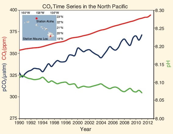
A smoothed time series of atmospheric CO2 mole fraction (in ppm) at the atmospheric Mauna Loa Observatory (top red line), surface ocean partial pressure of CO2 (pCO2; middle blue line) and surface ocean pH (bottom green line) at Station ALOHA in the subtropical North Pacific north of Hawaii for the period from 1990–2011. The results indicate that the surface ocean pCO2 trend is generally consistent with the atmospheric increase but is more variable due to large-scale interannual variability of oceanic processes.
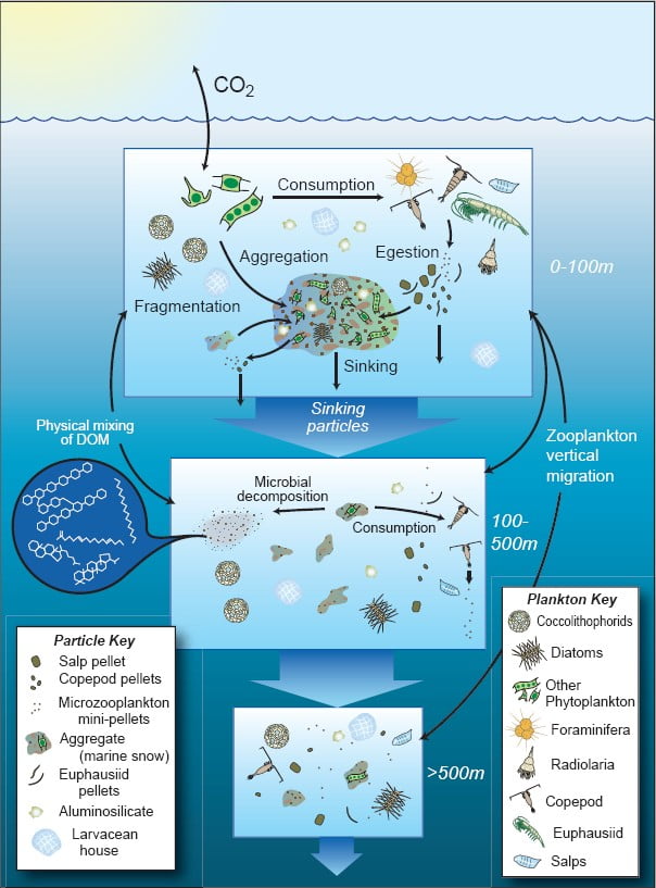
The Ocean’s Biological Pump
WG2 chapter 6 figure 4
The ocean’s biological pump is one way in which carbon can be captured and deposited. Given the available science, it is difficult to know exactly how the pump may be altered by climate change and whether it would present a positive or negative feedback to climate change. Changes will affect, for example, grazing rates by larger fauna on the plankton, the depth at which various fauna live and changes to the speeds at which bacteria decompose material.
The ocean’s biological pump is one way in which carbon can be captured and deposited. Given the available science, it is difficult to know exactly how the pump may be altered by climate change and whether it would present a positive or negative feedback to climate change. Changes will affect, for example, grazing rates by larger fauna on the plankton, the depth at which various fauna live and changes to the speeds at which bacteria decompose material.
Biological Pump: The process of transporting carbon from the ocean’s surface layers to the deep ocean by the primary production of marine phytoplankton, which converts dissolved inorganic carbon (DIC), mainly CO2, and nutrients into organic matter through photosynthesis.
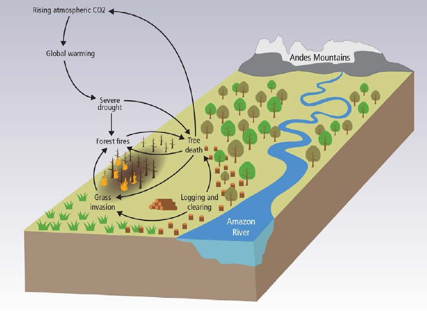
Questions to consider: State three factors which would cause a change to the Amazonian Forest Ecosystem. Explain the impact of the change to the Amazonian Forest Ecosystem When looking at the effect of climate change on ecosystems, why does the level of carbon dioxide in the atmosphere need to be considered as well as temperature change.
Climate change can affect terrestrial and marine ecosystems which in turn has impacts on both the water and carbon cycles and then feeds back to the climate.
Direct human influence on vegetation can also lead to impacts on the climate, through the energy, water and carbon cycles.
Both changes in carbon dioxide and changes in climate have impacts on vegetation.
The interactive effects of elevated CO2 and other global changes (such as climate change, nitrogen deposition and biodiversity loss) on ecosystem function are extremely complex.
Extreme weather events can have long lasting impacts on vegetation and the carbon and water cycles.
In general, climate exerts a dominant control over the distribution of terrestrial vegetation and surface properties that in turn affects the local climate by changing the local atmospheric water, Carbon and energy budgets. It has been hypothesized that these vegetation–climate feedbacks can explain shifts of vegetation through time: Firstly, increased transpiration may result in more precipitation, which in turn increases plant productivity, which amplifies transpiration further. Secondly, increased productivity leads to more canopy cover, which is darker (lower albedo) than snow and bare soil. This results in higher temperatures on the above ground parts of individual plants, thus also amplifying plant productivity.
The combined effects of a warming climate, higher levels of CO2, land-use change and increased Nitrogen availability may be responsible for primary productivity increases in many parts of the world. Enhanced productivity can lead to shifts in albedo and transpiration, which feed back to the water cycle through heat fluxes and precipitation.
Rising atmospheric CO2 concentrations affect ecosystems directly including through biological and chemical processes such as the carbon dioxide fertilisation effect. Plants can respond to elevated CO2 by opening their stomata less to take in the same amount of CO2 or by structurally adapting their stomatal density and size, both potentially reducing transpiration which increases the water efficiency of the plants but reduces the flow of water vapour, and the energy that goes with it, to the atmosphere. Paleo records over the Late Quaternary (past million years) show that changes in the atmospheric CO2 content between 180 and 280 ppmv had ecosystem-scale effects worldwide.
The direct effect of CO2 on plant physiology, independent of its role as a greenhouse gas, means that assessing climate change impacts on ecosystems and hydrology solely in terms of global mean temperature rise is an oversimplification. A 2°C rise in global mean temperature, for example, may have a different net impact on ecosystems depending on the change in CO2 concentration accompanying the rise: If a small change in CO2 causes a 2°C rise, or, if other greenhouse gases are mainly responsible for the rise, the vegetation response will be different to a 2°C rise triggered by a large increase in CO2.
Vegetation cover can be affected by climate change, with forest cover potentially decreasing (e.g. in the tropics) or increasing (e.g. in high latitudes). In particular, the Amazon forest has been the subject of several studies, generally agreeing that future climate change would increase the risk of tropical forest being replaced by seasonal forest or even savannah. The increase in atmospheric CO2 reduces the risk, through an increase in the water efficiency of plants.
Direct human changes to the land cover can also have impacts on the carbon and water cycles, as well as on the Earth’s energy balance, through changes in surface albedo, transpiration and evaporation.
The coupling processes between terrestrial Carbon, Nitrogen and hydrological processes are extremely complex and far from well understood.
The effect of climate extremes on vegetation and the carbon and water cycles Extreme events such as heatwaves, droughts and storms can cause vegetation death, fires and subsequent insect infestations which actually lead to a net output of carbon from ecosystems. For example, forests are characterized by the large biomass carbon stocks, which are vulnerable to wind damage, storms, ice storms, frost, drought, fire and pathogen or pest outbreaks. Trees take a long time to regrow, so the recovery times for forest biomass lost through extreme events are particularly long. Therefore, the effects of climate extremes on the carbon balance in forests are both immediate and lagged, and potentially long-lasting. Climate extremes may also trigger processes that decrease the turnover rate of some carbon pools and lead to additional long-term sequestration in these pools. A well-known example is charcoal created in fires, which generally persists longer in soils than leaf litter.
During the European 2003 heatwave, it was the lack of precipitation (and soil moisture) rather than the high temperatures which was the main factor limiting vegetation growth in the temperate and Mediterranean forest ecosystems.
How do land-use and land-cover changes cause changes in climate? WG2 FAQ 4.1
Land use change affects the local as well as the global climate. Different forms of land cover and land use can cause warming or cooling and changes in rainfall, depending on where they occur in the world, what the preceding land cover was, and how the land is now managed. Vegetation cover, species composition and land management practices (such as harvesting, burning, fertilizing, grazing or cultivation) influence the emission or absorption of greenhouse gases. The brightness of the land cover affects the fraction of solar radiation that is reflected back into the sky, instead of being absorbed, thus warming the air immediately above the surface. Vegetation and land use patterns also influence water use and evapotranspiration, which alter local climate conditions. Effective land-use strategies can also help to mitigate climate change.
What are the non-greenhouse gas effects of rising carbon dioxide on ecosystems? WG2 FAQ 4.2
Carbon dioxide (CO2) is an essential building block of the process of photosynthesis. Simply put, plants use sunlight and water to convert CO2 into energy. Higher CO2 concentrations enhance photosynthesis and growth (up to a point), and reduce the water used by the plant. This means that water remains longer in the soil or recharges rivers and aquifers. These effects are mostly beneficial; however, high CO2 also has negative effects, in addition to causing global warming. High CO2 levels cause the nitrogen content of forest vegetation to decline and can increase their chemical defences, reducing their quality as a source of food for plant-eating animals. Furthermore, rising CO2 causes ocean waters to become acidic, and can stimulate more intense algal blooms in lakes and reservoirs.
The Carbon Dioxide fertilisation effect WG1 Box 6.3
Elevated atmospheric CO2 concentrations lead to higher leaf photosynthesis and reduced canopy transpiration, which in turn lead to increased plant water use efficiency and reduced fluxes of latent heat from the surface to the atmosphere. The increase in leaf photosynthesis with rising CO2, the so-called CO2 fertilisation effect, plays a dominant role in terrestrial biogeochemical models to explain the global land carbon sink, yet it is one of most unconstrained process in those models.
Field experiments provide a direct evidence of increased photosynthesis rates and water use efficiency (plant carbon gains per unit of water loss from transpiration) in plants growing under elevated CO2. These physiological changes translate into a broad range of higher plant carbon accumulation in more than two-thirds of the experiments and with increased net primary productivity (NPP) of about 20 to 25% at double CO2 from pre-industrial concentrations. Since the last IPCC report, new evidence is available from long-term Free-air CO2 Enrichment (FACE) experiments in temperate ecosystems showing the capacity of ecosystems exposed to elevated CO2 to sustain higher rates of carbon accumulation over multiple years. However, FACE experiments also show the diminishing or lack of CO2 fertilisation effect in some ecosystems and for some plant species. This lack of response occurs despite increased water use efficiency, also confirmed with tree ring evidence
Nutrient limitation is hypothesized as primary cause for reduced or lack of CO2 fertilisation effect observed on NPP in some experiments. Nitrogen and phosphorus are very likely to play the most important role in this limitation of the CO2 fertilisation effect on NPP, with nitrogen limitation prevalent in temperate and boreal ecosystems, and phosphorus limitation in the tropics. Micronutrients interact in diverse ways with other nutrients in constraining NPP such as molybdenum and phosphorus in the tropics. Thus, with high confidence, the CO2 fertilisation effect will lead to enhanced NPP, but significant uncertainties remain on the magnitude of this effect, given the lack of experiments outside of temperate climates.
A Possible Amazon Basin Tipping Point WG2 Box 4.3
Since the last assessment report of the IPCC (AR4), our understanding of the potential of a large-scale, climate-driven, self-reinforcing transition of Amazon forests to a dry stable state (known as the Amazon “forest dieback”) has improved. Modelling studies indicate that the likelihood of a climate-driven forest dieback by 2100 is lower than previously thought, although lower rainfall and more severe drought is expected in the eastern Amazon. There is now medium confidence that climate change alone (that is, through changes in the climate envelope, without invoking fire and land use) will not drive large-scale forest loss by 2100 although shifts to drier forest types are predicted in the eastern Amazon.
Meteorological fire danger is projected to increase. Field studies and regional observations have provided new evidence of critical ecological thresholds and positive feedbacks between climate change and land-use activities that could drive a fire mediated, self-reinforcing dieback during the next few decades. There is now medium confidence that severe drought episodes, land use, and fire interact synergistically to drive the transition of mature Amazon forests to low-biomass, low-statured fire-adapted woody vegetation. Most primary forests of the Amazon Basin have damp fine fuel layers and low susceptibility to fire, even during annual dry seasons. Forest susceptibility to fire increases through canopy thinning and greater sunlight penetration caused by tree mortality associated with selective logging, previous forest fire, severe drought, or drought-induced tree mortality. The impact of fire on tree mortality is also weather-dependent. Under very dry, hot conditions, fire-related tree mortality can increase. Under some circumstances, tree damage is sufficient to allow light-demanding, flammable grasses to establish in the forest understorey, increasing forest susceptibility to further burning. There is high confidence that logging, severe drought, and previous fire increase Amazon forest susceptibility to burning. Landscape level processes further increase the likelihood of forest fire. Fire ignition sources are more common in agricultural and grazing lands than in forested landscapes, and forest conversion to grazing and crop lands can inhibit regional rainfall through changes in albedo and evapotranspiration or through smoke that can inhibit rainfall under some circumstances. Apart from these landscape processes, climate change could increase the incidence of severe drought episodes.
If recent patterns of deforestation (through 2005), logging, severe drought, and forest fire continue into the future, more than half of the region’s forests will be cleared, logged, burned or exposed to drought by 2030, even without invoking positive feedbacks with regional climate, releasing 20±10 Pg of carbon to the atmosphere. The likelihood of a tipping point being reached may decline if extreme droughts (such as 1998, 2005, and 2010) become less frequent, if land management fires are suppressed, if forest fires are extinguished on a large scale, if deforestation declines, or if cleared lands are reforested. The 77% decline in deforestation in the Brazilian Amazon with 80% of the region’s forest still standing demonstrates that policy-led avoidance of a fire-mediated tipping point is plausible.
WG2 Chapter 4, Figure 8. The forests of the Amazon Basin are being altered through severe droughts, land use (deforestation, logging), and increased frequencies of forest fire. Some of these processes are self-reinforcing through positive feedbacks, and create the potential for a large-scale tipping point. For example, forest fire kills trees, increasing the likelihood of subsequent burning. This effect is magnified when tree death allows forests to be invaded by grasses, which are more flammable. Deforestation provides ignition sources to flammable forests, contributing to this dieback. Climate change contributes to this tipping point by increasing drought severity, reducing rainfall and raising air temperatures, particularly in the eastern Amazon Basin.
Vegetation changes in the Amazon basin
WG2 Chapter 4, Figure 8. The forests of the Amazon Basin are already being altered through severe droughts, changes in land use (deforestation, logging), and increased frequencies of forest fire. Some of these processes are self-reinforcing through positive feedbacks, and create the potential for a large-scale tipping point. For example, forest fire kills trees, increasing the likelihood of subsequent burning. This effect is magnified when tree death allows forests to be invaded by flammable grasses. Deforestation provides ignition sources to flammable forests, contributing to this dieback. Climate change contributes to this tipping point by increasing drought severity, reducing rainfall and raising air temperatures, particularly in the eastern Amazon Basin.
There is a high risk that the large magnitudes and high rates of climate change this century will result in abrupt and irreversible regional-scale changes to terrestrial and freshwater ecosystems, especially in the Amazon and Arctic, leading to additional climate change.
There are plausiblemechanisms, supported by experimental evidence, observations, and climate model simulations, for the existence of ecosystem tipping points in the rainforests of the Amazon basin. Climate change (temperature and precipitation changes) alone isnot projected to lead to abrupt widespread loss of forest cover in the Amazon during this century. However, a projected increase in severe drought episodes, related to stronger El Niño events, together with land-use change and forest fires,would cause much of the Amazon forest to transform to less dense, drought- and fire-adapted ecosystems. This would risk reducing biodiversity in an important ecosystem, and would reduce the amount of carbon absorbed from the atmosphere through photosynthesis. It would also reduce the amount of evaporation, increasing the warming locally. Large reductions in deforestation, as well as wider application of effective wildfiremanagement would lower the risk of abrupt change in the Amazon.
Amazonian forests were estimated to have lost 1.6 PgC and 2.2 PgC following the severe droughts of 2005 and 2010, respectively.
Climate extremes and the carbon cycle, M. Reichstein, M. Bahn, P. Ciais, D. Frank, M. Mahecha, S. Seneviratne,.J. Zscheischler, C. Beer, N. Buchmann, D. Frank, D. Papale, A. Rammig, P. Smith, K. Thonicke, M. van der Velde, S. Vicca, A. Walz & M. Wattenbach, 2013, 500, Nature, 287-295.
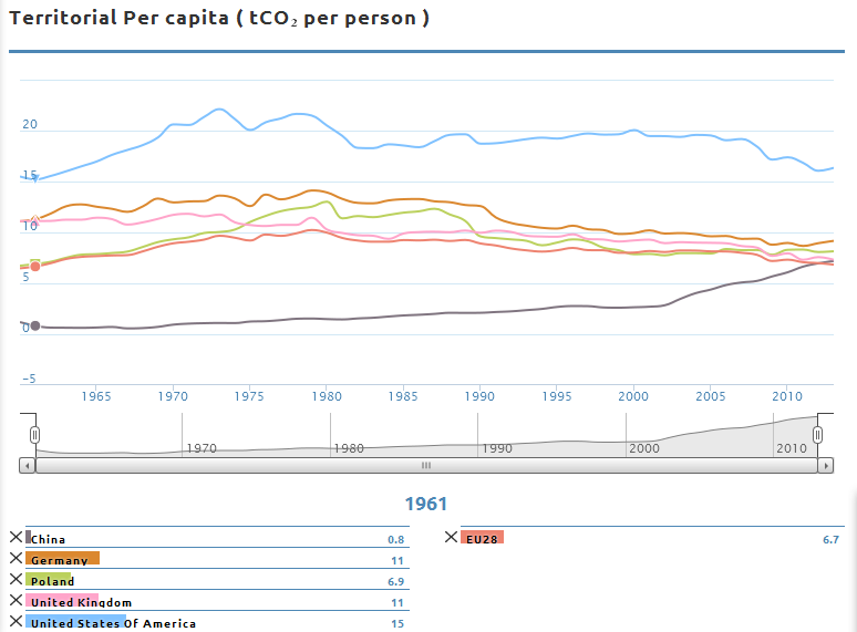
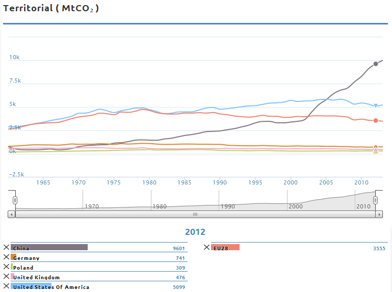
Carbon Emissions Map, resizing the territories according to their proportion of global carbon dioxide emissions and colouring them according to their per capita emissions.
Reproduced with permission from Dr. Benjamin Hennig http://www.viewsoftheworld.net/ .
Questions to consider:Describe the global distribution of carbon emissions Explain the reasons for the high proportion of global carbon dioxide emissions for one country shown on the carbon emissions map.
Carbon Emissions Map, resizing the territories according to their proportion of global carbon dioxide emissions and colouring them according to their per capita emissions.
Reproduced with permission from Dr. Benjamin Hennig http://www.viewsoftheworld.net/ .
Summary:
The increase in CO2 emissions from both fossil fuel burning and land use change are the dominant cause of the observed increase in atmospheric CO2 concentration, which is now over 40% above pre-industrial levels.
Global CO2 emissions have continued to grow over the last 10 years, but there are large variations in emission trajectories between countries.
The Ocean has absorbed about 30% of the emitted anthropogenic carbon dioxide.
Anthropogenic CO2 emissions are currently closest to the highest emissions scenario the IPCC considered.
Figure reproduced with permission from the Global Carbon Atlas: globalcarbonatlas.org Data sources CDIAC: Boden, TA, G Marland, and RJ Andres. 2013. Global, Regional, and National Fossil-Fuel CO2 Emissions. Carbon Dioxide Information Analysis Center (CDIAC), Oak Ridge National Laboratory, US Department of Energy, Oak Ridge, Tenn., USA doi:10.3334/CDIAC/00001_V2013 http://cdiac.ornl.gov/trends/emis/meth_reg.html and UN: United Nations Population Division – World Population Prospects: The 2012 Revision, 2013 http://esa.un.org/unpd/wpp/Excel-Data/population.htm
Annual anthropogenic CO2 emissions and their partitioning among the atmosphere, land and ocean (PgC yr–1) from 1750 to 2011. (Top) Fossil fuel and cement CO2 emissions by category (Bottom) Fossil fuel and cement CO2 emissions, CO2 emissions from net land use change (mainly deforestation), the atmospheric CO2 growth rate, the ocean CO2 sink and the residual land sink which represents the sink of anthropogenic CO2 in natural land ecosystems. The emissions and their partitioning only include the fluxes that have changed since 1750, and not the natural CO2 fluxes (e.g., atmospheric CO2 uptake from weathering, outgassing of CO2 from lakes and rivers, and outgassing of CO2 by the ocean from carbon delivered by rivers) between the atmosphere, land and ocean reservoirs that existed before that time and still exist today. WG1 Chapter 6, Figure 8.
Anthropogenic CO2 emissions to the atmosphere were 555 ± 85 PgC between 1750 and 2011. Of this, fossil fuel combustion and cement production contributed 375 ± 30 PgC and land use change (including deforestation, afforestation (planting new forest) and reforestation) contributed 180 ± 80 PgC. In 2002–2011, average fossil fuel and cement manufacturing emissions were 7.6 to 9.0 PgC/ year, with an average increase of 3.2%/ year compared with 1.0%/ year during the 1990s. In 2011, fossil fuel emissions were in the range of 8.7 to 10.3 PgC.
Emissions due to land use changes between 2002 and 2011 are dominated by tropical deforestation, and are estimated to range between 0.1 to 1.7 PgC/year. This includes emissions from deforestation of around 3 PgC/ year compensated by an uptake of around 2 PgC/year by forest regrowth (mainly on abandoned agricultural land). The IPCC concluded that the increase in CO2 emissions from both fossil fuel burning and land use change are the dominant cause of the observed increase in atmospheric CO2 concentration.
Reducing greenhouse gas emissions in Germany, an Advanced Country (AC)
Between 1990 and 2014, most major German sources of emissions achieved CO2 reductions. In the energy industry sector, which is responsible for the largest share (around 40%) of Germany’s greenhouse gas emissions, emissions fell by 24% between 1990 and 2014. Even bigger reductions were achieved by households (32.9 %) and industry (33.8 %), helped by the fall of the Berlin wall and the subsequent decline of East German industry and power production and the 2009 economic crisis. The transport sector only reduced its emissions by 0.2 %. Around half of German electricity is still produced in coal- and gas-fired power plants but Germany is pushing ahead with its transition to renewable energy sources. The production costs of renewable energy have dropped by 70% in the past 5 years, making them a much more competitive energy source. In 2015 the share of renewables in the country’s domestic energy mix increased to 33%, At the same time, Germany managed to cut down its power consumption in the past year by 3.8%, despite a booming economy (+1.4 %) which generally translates into a higher energy demand, by using LED technology and energy saving measures. CO2 emissions correspondingly fell by 5%. However, 4% of that figure is linked to mild weather conditions requiring less heating. In 2011, Germany took 8 nuclear power plants off the grid after the Fukushima disaster. Germany aims to cut greenhouse gas emissions by 40% by 2020 and up to 95% in 2050. It may struggle to meet those targets. Additional Sources: https://www.cleanenergywire.org/factsheets/germanys-greenhouse-gas-emissions-and-climate-targets , http://www.dw.com/en/renewables-help-cut-german-co2-emissions/a-18176835
Reducing greenhouse gas emissions in the USA, an Advanced Country (AC)
Until 2006, when it was overtaken by China, the USA was the largest emitter of greenhouse gases. The largest contributor to U.S. greenhouse gas emissions is carbon dioxide from fossil fuel combustion. Changes in this are influenced by many long-term and short-term factors, including population and economic growth, energy price fluctuations, technological changes and the mix of fuels used for electricity generation, short term economic conditions and the weather. U.S. emissions increased by 5.9 % from 1990 to 2013. From 2010 to 2011, CO2 emissions from fossil fuel combustion decreased by 2.5 % due to: (1) a decrease in coal consumption, with increased natural gas consumption and a significant increase in hydropower used; (2) a decrease in transportation-related energy consumption due to higher fuel costs, improvements in fuel efficiency, and a reduction in miles travelled; and (3) relatively mild winter conditions resulting in an overall decrease in energy demand in most sectors. From 2011 to 2012, CO2 emissions from fossil fuel combustion decreased by 3.9 %, with emissions from fossil fuel combustion at their lowest level since 1994 due to:
(1) a slight increase in the price of coal, and a significant decrease in the price of natural gas; (2) the weather conditions, with no extremely hot days in the summer and much warmer than usual winter temperatures leading to heating degree days decreasing by 12.6 %. This decrease in heating degree days resulted in a decreased demand for heating fuel in the residential and commercial sector, which had a decrease in natural gas consumption of 11.7 and 8.0 %, respectively.
From 2012 to 2013, CO2 emissions from fossil fuel combustion increased by 2.6 % due to: (1) the weather – heating degree days increased 18.5 % in 2013 compared to 2012. (2)The consumption of natural gas used to generate electricity decreased by 10.2 % due to an increase in the price of natural gas. Electric power plants shifted some consumption from natural gas to coal, increasing coal consumption to generate electricity by 4.2 %.
The use of fracking to extract natural gas is expected to reduce American emissions in the future, by reducing its reliance on coal.
Reducing greenhouse gas emissions in China, an Emerging and Developing Country (EDC
Source: Wikipedia https://en.wikipedia.org/wiki/Economic_history_of_China_(1949–present) Scatter graph of the People’s Republic of China’s GDP between 1952 to 2005, based on publicly available nominal GDP data published by the People’s Republic of China and compiled by Hitotsubashi University (Japan) and confirmed by economic indicator statistics from the World Bank.
China’s emissions started to climb in the 1950s as its economy grew – at an average rate of 10% per year during the period 1990–2004. Over the past 20 years huge numbers of mainly coal fired power stations have been constructed. In 2003, following legislation to protect private property rights, construction boomed and current rates of housing construction are equivalent to building a city the size of Rome in 2 weeks! China’s total emissions overtook those of the USA in 2006 and its emissions per head of population overtook those of the EU in 2014. In China, manufacturing and construction account for two thirds of emissions by source (one third of that is steel production, a quarter is cement, chemicals and plastics produce 17%, aluminium and other metals a further 13%) .Unlike most countries, household efficiency is relatively unimportant but sustainable industry is a big priority. It is worth noting that about 20% of Chinese emissions arise from producing clothes, furniture and even solar panels that are shipped to Europe and America.
In the first third of 2015, China dramatically cut its carbon dioxide emissions, with its reduction equalling the UK’s total emissions for the same period. This is largely due to the closure of more than 1,000 coal mines; coal output is down 7.4% year on year. By 2020, China hopes to reduce coal from around 66% of its energy consumption to 62% which should also improve air quality.
China will aim to cut its greenhouse gas emissions per unit of gross domestic product by 60-65% from 2005 levels under a plan submitted to the United Nations for the 2015 COP21 meeting in Paris. China said it would increase the share of non-fossil fuels (wind and solar) as part of its primary energy consumption to about 20% by 2030, and peak emissions by around the same point, though it would “work hard” to do so earlier. Indeed, China is now the world’s largest investor in renewable sources of energy.
Reducing greenhouse gas emissions in Poland, an Emerging and Developing Country (EDC)
Poland is not among the largest emitters of greenhouse gases globally (its share is just 1%), but its economy is among the least carbon-efficient in the EU. Among transition economies, Poland’s performance appears better: its carbon intensity on a per capita basis is situated in about the middle of the countries of Eastern and Central Europe and Central Asia. In 2007, around 1.3 metric tonnes of CO2eq, 1.3tCO2eq, were required to produce €1 million in GDP, while the EU average was less than 0.5 tC02eq.
Poland cut its emissions considerably as a side effect of the transition to a market economy, greenhouse gas emissions collapsed along with output through the 90s (declining 20%), as inefficient, often highly energy-intensive plants shut down during the early years of transition. The period of 1996 to 2002 witnessed another 17 % decline in emissions despite GDP increasing. Overall, although Poland’s GDP nearly doubled from 1988 to 2008, its GHG emissions were reduced by about 30%. During the last half decade or so, a more traditional positive correlation between GDP growth and GHG emissions has re-established itself.
Poland depends on domestically available coal far more than other EU countries (solid fuels, coal and lignite, constitute 57% of gross inland energy consumption for heat and electricity) with very little renewable energy production and no nuclear power. This reliance on coal makes future emission reduction challenging.
Transport, which contributes about 10% of overall GHG emissions, has grown by almost three-quarters since transition, with a very high share of used vehicles, which tend to be much more fuel inefficient and polluting. However, Poland still has relatively low rates of motorisation, suggesting that the growth of road transport could be high in the future. Poland has made considerable advances in energy efficiency in the past 20 years; yet further efforts are required to bring it to Western European standards.
In 2014, the EU pledged a 40% reduction in greenhouse gas emissions by 2030. To help some countries achieve this, concessions including carbon credits and emissions allowances were made. Poland claimed 60% of the concessions available to 2019, which it will be able to sell to other EU countries, on the condition that it spends the proceeds on diversifying its energy mix and modernising its coal fired power stations.


