WG2 – Impacts, Adaptation and Vulnerability
- How will climate change affect the frequency and severity of floods and droughts?
- How will the availability of water resources be affected by climate change?
- How should water management be modified in the face of climate change?
- Does climate change imply only bad news about water resources?
- How do land-use and land-cover changes cause changes in climate?
- What are the non-greenhouse gas effects of rising carbon dioxide on ecosystems?
- Will the number of invasive alien species increase due to climate change?
- How does climate change contribute to species extinction?
- Why does it matter if ecosystems are altered by climate change?
- Can ecosystems be managed to help them and people to adapt to climate change?
- What are the economic costs of changes in ecosystems due to climate change?
- How does climate change affect coastal marine ecosystems?
- How is climate change influencing coastal erosion?
- How can coastal communities plan for and adapt to the impacts of climate change, in particular sea level rise?
- Why are climate impacts on oceans and their ecosystems so important?
- What is different about the effects of climate change on the oceans compared to the land, and can we predict the consequences?
- Why are some marine organisms affected by ocean acidification?
- What changes in marine ecosystems are likely because of climate change?
- What factors determine food security and does low food production necessarily lead to food insecurity?
- How could climate change interact with change in fish stocks, ocean acidification?
- How could adaptation actions enhance food security and nutrition?
- Do experiences with disaster risk reduction in urban areas provide useful lessons for climate-change adaptation?
- As cities develop economically, do they become better adapted to climate change?
- Does climate change cause urban problems by driving migration from rural to urban areas?
- Shouldn’t urban adaptation plans wait until there is more certainty about local climate change impacts?
- What is distinctive about rural areas in the context of climate change impacts, vulnerability and adaptation?
- What will be the major climate change impacts in rural areas across the world?
- What will be the major ways in which rural people adapt to climate change?
- Why are key economic sectors vulnerable to climate change?
- How does climate change impact insurance and financial services?
- Are other economic sectors vulnerable to climate change too?
- How does climate change affect human health?
- Will climate change have benefits for health?
- Will climate change introduce new infectious diseases into Europe?
- Who is most affected by climate change?
- What is the most important adaptation strategy to reduce the health impacts of climate change?
- What are health “co-benefits” of climate change mitigation measures?
- What are the principal threats to human security from climate change?
- Can lay knowledge of environmental risks help adaptation to climate change?
- How many people could be displaced as a result of climate change?
- What role does migration play in adaptation to climate change, particularly in vulnerable regions?
- Will climate change cause war between countries?
- What are multiple stressors and how do they intersect with inequalities to influence livelihood trajectories?
- How important are climate change-driven impacts on poverty compared to other drivers of poverty?
- Are there unintended negative consequences of climate change policies for people who are poor?
- Why do the precise definitions about adaptation activities matter?
- What is the present status of climate change adaptation planning and implementation across the globe?
- What types of approaches are being used in adaptation planning and implementation?
- What is the difference between an adaptation barrier, constraint, obstacle, and limit?
- What opportunities are available to facilitate adaptation?
- How does greenhouse gas mitigation influence the risk of exceeding adaptation limits?
- Given the significant uncertainty about the effects of adaptation measures, can economics contribute much to decision-making in this area?
- Could economic approaches bias adaptation policy and decisions against the interests of the poor, vulnerable populations, or ecosystems?
- In what ways can economic instruments facilitate adaptation to climate change in developed and developing countries?
- Why are detection and attribution of climate impacts important?
- Why is it important to assess impacts of all climate change aspects, and not only impacts of anthropogenic climate change?
- What are the main challenges in detecting climate change impacts?
- What are the main challenges in attributing changes in a system to climate change?
- Is it possible to attribute a single event, like a disease outbreak or the extinction of a species, to climate change?
- Does science provide an answer to the question of how much warming is unacceptable?
- How does climate change interact with and amplify pre-existing risks?
- How can climate change impacts on one region cause impacts on other distant areas?
- What is a climate-resilient pathway for development?
- What do you mean by” transformational changes”?
- Why are climate-resilient pathways needed for sustainable development?
- Are there things that we can be doing now that will put us on the right track toward climate-resilient pathways?
- How does this report stand alongside previous assessments for informing regional adaptation?
- Do local and regional impacts of climate change affect other parts of the world?
- What regional information should I take into account for climate risk management for the 20 year time horizon?
- Is the highest resolution climate projection the best to use for performing impacts assessments?
- How could climate change impact food security in Africa?
- What role does climate change play with regard to violent conflict in Africa?
- Will I still be able to live on the coast in Europe?
- Will Europe need to import more food because of climate change?
- What will the projected impact of future climate change be on freshwater resources in Asia?
- How will climate change affect food production and food security in Asia?
- Who is most at risk from climate change in Asia?
- How can we adapt to climate change if projected future changes remain uncertain?
- What are the key risks from climate change to Australia and New Zealand?
- What impact is climate having on North America?
- Can adaptation reduce the adverse impacts of climate in North America?
- What is the impact of glacier retreat on natural and human systems in the tropical Andes?
- Can payment for ecosystem services (PES) be used as an effective way to help local communities adapt to climate change?
- Are there emerging and re emerging human diseases as a consequence of climate variability and change in the region?
- What will be the net socio-economic impacts of change in the polar regions?
- Why are changes in sea ice so important to the polar regions?
- Why is it difficult to detect and attribute changes on small islands to climate change?
- Why is the cost of adaptation to climate change so high in small islands?
- Is it appropriate to transfer adaptation and mitigation strategies between and within small island countries and regions?
- Can we reverse the climate change impacts on the ocean?
- Does slower warming mean less impact on plants and animals?
- How will marine primary productivity change?
- Will climate change cause ‘dead zones’ in the oceans?
- How can we use non-climate factors to manage climate change impacts on the oceans?
- On what information is the new assessment based, and how has that information changed since the last report, the IPCC Fourth Assessment Report in 2007?
- How is the state of scientific understanding and uncertainty communicated in this assessment?
- How has our understanding of the interface between human, natural,and climate systems expanded since the 2007 IPCC Assessment?
- What constitutes a good (climate) decision?
- Which is the best method for climate change decision-making/assessing adaptation?
- Is climate change decision-making different from other kinds of decision-making?
WG3 Mitigation of Climate Change
- What is climate change mitigation?
- What causes GHG emissions?
- When is uncertainty a reason to wait and learn rather than acting now in relation to climate policy and risk management strategies?
- How can behavioural responses and tools for improving decision impact on climate change policy?
- How does the presence of uncertainty affect the choice of policy instruments?
- What are the uncertainties and risks that are of particular importance to climate policy in developing countries?
- The IPCC is charged with providing the world with a clear scientific view of the current state of knowledge on climate change. Why does it need to consider ethics?
- Do the terms justice, fairness and equity mean the same thing?
- What factors are relevant in considering responsibility for future measures that would mitigate climate change?
- Why does the IPCC need to think about sustainable development?
- The IPCC and UNFCCC focus primarily on GHG emissions within countries. How can we properly account for all emissions related to consumption activities, even if these emissions occur in other countries?
- What kind of consumption has the greatest environmental impact?
- Why is equity relevant in climate negotiations?
- Based on trends in the recent past, are GHG emissions expected to continue to increase in the future, and if so, at what rate and why?
- Why is it so hard to attribute causation to the factors and underlying drivers influencing GHG emissions?
- What options, policies, and measures change the trajectory of GHG emissions?
- What considerations constrain the range of choices available to society and their willingness or ability to make choices that would contribute to lower GHG emissions?
- Is it possible to bring climate change under control given where we are and what options are available to us? What are the implications of delaying mitigation or limits on technology options?
- What are the most important technologies for mitigation? Is there a silver bullet technology?
- How much would it cost to bring climate change under control?
- How much does the energy supply sector contribute to the GHG emissions?
- What are the main mitigation options in the energy supply sector?
- What barriers need to be overcome in the energy supply sector to enable a transformation to low‐GHG emissions?
- How much does the transport sector contribute to GHG emissions and how is this changing?
- What are the main mitigation options and potentials for reducing GHG emissions?
- Are there any co‐benefits associated with mitigation actions?
- What are the recent advances in building sector technologies and know-how since the AR4 that are important from a mitigation perspective?
- How much could the building sector contribute to ambitious climate change mitigation goals, and what would be the costs of such efforts?
- Which policy instrument(s) have been particularly effective and/or cost-effective in reducing building‐sector GHG emission (or their growth, in developing countries)
- How much does the industry sector contribute to GHG emissions?
- What are the main mitigation options in the industry sector and what is the potential for reducing GHG emissions?
- How will the level of product demand, interactions with other sectors, and collaboration within the industry sector affect emissions from industry?
- What are the barriers to reducing emissions in industry and how can these be overcome? Are there any co‐benefits associated with mitigation actions in industry?
- How much does Agriculture, Forestry and Other Land Use (AFOLU) contribute to GHG emissions and how is this changing?
- How will mitigation actions in AFOLU affect GHG emissions over different timescales?
- What is the potential of the main mitigation options in AFOLU for reducing GHG emissions?
- Are there any co‐benefits associated with mitigation actions in AFOLU?
- What are the barriers to reducing emissions in AFOLU and how can these be overcome?
- Why is the IPCC including a new chapter on human settlements and spatial planning? Isn’t this covered in the individual sectoral chapters?
- What is the urban share of global energy and GHG emissions?
- What is the potential of human settlements to mitigate climate change?
- Given that GHG emissions abatement must ultimately be carried out by individuals and firms within countries, why is international cooperation necessary?
- What are the advantages and disadvantages of including all countries in international cooperation on climate change (an ‘inclusive’ approach) and limiting participation (an ‘exclusive’ approach)?
- What are the options for designing policies to make progress on international cooperation on climate change mitigation?
- How are regions defined in the AR5?
- Why is the regional level important for analyzing and achieving mitigation objectives?
- How do opportunities and barriers for mitigation differ by region?
- What role can and does regional cooperation play to mitigate climate change?
- What kind of evidence and analysis will help us design effective policies?
- What is the best climate change mitigation policy?
- What is climate finance?
- How much investment and finance is currently directed to projects that contribute to mitigate climate change and how much extra flows will be required in the future to stay below the 2°C limit?
Are risks of climate change mostly due to changes in extremes, changes in average climate, or both?
People and ecosystems across the world experience climate in many different ways, but weather and climate extremes strongly influence losses and disruptions. Average climate conditions are important. They provide a starting point for understanding what grows where and for informing decisions about tourist destinations, other business opportunities, and crops to plant. But the impacts of a change in average conditions often occur as a result of changes in the frequency, intensity, or duration of extreme weather and climate events. It is the extremes that place excessive and often unexpected demands on systems poorly equipped to deal with those extremes. For example, wet conditions lead to flooding when storm drains and other infrastructure for handling excess water are overwhelmed. Buildings fail when wind speeds exceed design standards. For many kinds of disruption, from crop failure caused by drought to sickness and death from heat waves, the main risks are in the extremes, with changes in average conditions representing a climate with altered timing, intensity, and types of extremes.
How much can we say about what society will be like in the future, in order to plan for climate change impacts?
Overall characteristics of societies and economies, such as population size, economic activity, and land use, are highly dynamic. On the scale of just one or two decades, and sometimes in less time than that, technological revolutions, political movements, or singular events can shape the course of history in unpredictable ways. To understand potential impacts of climate change for societies and ecosystems, scientists use scenarios to explore implications of a range of possible futures. Scenarios are not predictions of what will happen, but they can be useful tools for researching a wide range of “what if” questions about what the world might be like in the future. They can be used to study future emissions of greenhouse gases and climate change. They can also be used to explore the ways climate-change impacts depend on changes in society, such as economic or population growth or progress in controlling diseases. Scenarios of possible decisions and policies can be used to explore the solution space for reducing greenhouse gas emissions and preparing for a changing climate. Scenario analysis creates a foundation for understanding risks of climate change for people, ecosystems, and economies across a range of possible futures. It provides important tools for smart decision-making when both uncertainties and consequences are large.
Why is climate change a particularly difficult challenge for managing risk?
Risk management is easier for nations, companies, and even individuals when the likelihood and consequences of possible events are readily understood. Risk management becomes much more challenging when the stakes are higher or when uncertainty is greater. As the WGII AR5 demonstrates, we know a great deal about the impacts of climate change that have already occurred, and we understand a great deal about expected impacts in the future. But many uncertainties remain, and will persist. In particular, future greenhouse gas emissions depend on societal choices, policies, and technology advancements not yet made, and climate-change impacts depend on both the amount of climate change that occurs and the effectiveness of development in reducing exposure and vulnerability. The real challenge of dealing effectively with climate change is recognizing the value of wise and timely decisions in a setting where complete knowledge is impossible. This is the essence of risk management.
What are the timeframes for mitigation and adaptation benefits?
Adaptation can reduce damage from impacts that cannot be avoided. Mitigation strategies can decrease the amount of climate change that occurs, as summarized in the WGIII AR5. But the consequences of investments in mitigation emerge over time. The constraints of existing infrastructure, limited deployment of many clean technologies, and the legitimate aspirations for economic growth around the world all tend to slow the deviation from established trends in greenhouse gas emissions. Over the next few decades, the climate change we experience will be determined primarily by the combination of past actions and current trends. The near-term is thus an era where short-term risk reduction comes from adapting to the changes already underway. Investments in mitigation during both the near term and the longer-term do, however, have substantial leverage on the magnitude of climate change in the latter decades of the century, making the second half of the 21st century and beyond an era of climate options. Adaptation will still be important during the era of climate options, but with opportunities and needs that will depend on many aspects of climate change and development policy, both in the near-term and in the long-term.
Can science identify thresholds beyond which climate change is dangerous?
Human activities are changing the climate. Climate change impacts are already widespread and consequential. But while science can quantify climate change risks in a technical sense, based on the probability, magnitude, and nature of the potential consequences of climate change, determining what is dangerous is ultimately a judgment that depends on values and objectives. For example, individuals will value the present versus the future differently and will bring personal world views on the importance of assets like biodiversity, culture, and aesthetics. Values also influence judgments about the relative importance of global economic growth versus assuring the wellbeing of the most vulnerable among us. Judgments about dangerousness can depend on the extent to which one’s livelihood, community, and family are directly exposed and vulnerable to climate change. An individual or community displaced by climate change might legitimately consider that specific impact dangerous, even though that single impact might not cross the global threshold of dangerousness. Scientific assessment of risk can provide an important starting point for such value judgments about the danger of climate change.
Are we seeing impacts of recent climate change?
Yes, there is strong evidence of impacts of recent observed climate change on physical, biological, and human systems. Many regions have experienced warming trends and more frequent high-temperature extremes. Rising temperatures are associated with decreased snowpack, and many ecosystems are experiencing climate-induced shifts in the activity, range, or abundance of the species that inhabit them. Oceans are also displaying changes in physical and chemical properties that, in turn, are affecting coastal and marine ecosystems such as coral reefs, and other oceanic organisms such as mollusks, crustaceans, fishes, and zooplankton. Crop production and fishery stocks are sensitive to changes in temperature. Climate change impacts are leading to shifts in crop yields, decreasing yields overall and sometimes increasing them in temperate and higher latitudes, and catch potential of fisheries is increasing in some regions but decreasing in others. Some indigenous communities are changing seasonal migration and hunting patterns to adapt to changes in temperature.
Are the future impacts of climate change only negative? Might there be positive impacts as well?
Overall, the report identifies many more negative impacts than positive impacts projected for the future, especially for high magnitudes and rates of climate change. Climate change will, however, have different impacts on people around the world and those effects will vary not only by region but over time, depending on the rate and magnitude of climate change. For example, many countries will face increased challenges for economic development, increased risks from some diseases, or degraded ecosystems, but some countries will probably have increased opportunities for economic development, reduced instances of some diseases, or expanded arHow is climate change affecting monsoons?As cities develop economically, do they become better adapted to climate change? eas of productive land. Crop yield changes will vary with geography and by latitude. Patterns of potential catch for /a/lifis/aheries are changing globally as well, with both positive and negative consequences. Availability of resources such as usable water will also depend on changing rates of precipitation, with decreased availability in many places but possible increases in runoff and groundwater recharge in some regions like the high latitudes and wet tropics.
What communities are most vulnerable to the impacts of climate change?
Every society is vulnerable to the impacts of climate change, but the nature of that vulnerability varies across regions and communities, over time, and depends on unique socioeconomic and other conditions. Poorer communities tend to be more vulnerable to loss of health and life, while wealthier communities usually have more economic assets at risk. Regions affected by violence or governance failure can be particularly vulnerable to climate change impacts. Development challenges, such as gender inequality and low levels of education, and other differences among communities in age, race and ethnicity, socioeconomic status, and governance can influence vulnerability to climate change impacts in complex ways.
Does climate change cause violent conflicts?
Some factors that increase risks from violent conflicts and civil wars are sensitive to climate change. For example, there is growing evidence that factors like low per capita incomes, economic contraction, and inconsistent state institutions are associated with the incidence of civil wars, and also seem to be sensitive to climate change. Climate change policies, particularly those associated with changing rights to resources, can also increase risks from violent conflict. While statistical studies document a relationship between climate variability and conflict, there remains much disagreement about whether climate change directly causes violent conflicts.
How are adaptation, mitigation, and sustainable development connected?
Mitigation has the potential to reduce climate change impacts, and adaptation can reduce the damage of those impacts. Together, both approaches can contribute to the development of societies that are more resilient to the threat of climate change and therefore more sustainable. Studies indicate that interactions between adaptation and mitigation responses have both potential synergies and tradeoffs that vary according to context. Adaptation responses may increase greenhouse gas emissions (e.g., increased fossil-based air conditioning in response to higher temperatures), and mitigation may impede adaptation (e.g., increased use of land for bioenergy crop production negatively impacting ecosystems). There are growing examples of co-benefits of mitigation and development policies, like those which can potentially reduce local emissions of health-damaging and climate-altering air pollutants from energy systems. It is clear that adaptation, mitigation, and sustainable development will be connected in the future.
Why is it difficult to be sure of the role of climate change in observed effects on people and ecosystems?
Climate change is one of many factors impacting the Earth’s complex human societies and natural ecosystems. In some cases the effect of climate change has a unique pattern in space or time, providing a fingerprint for identification. In others, potential effects of climate change are thoroughly mixed with effects of land use change, economic development, changes in technology, or other processes. Trends in human activities, health, and society often have many simultaneous causes, making it especially challenging to isolate the role of climate change. Much climate-related damage results from extreme weather events and could be affected by changes in the frequency and intensity of these events due to climate change. The most damaging events are rare, and the level of damage depends on context. It can therefore be challenging to build statistical confidence in observed trends, especially over short time periods. Despite this, many climate change impacts on the physical environment and ecosystems have been identified, and increasing numbers of impacts have been found in human systems as well.
On what information is the new assessment based, and how has that information changed since the last report, the IPCC Fourth Assessment Report in 2007?
Thousands of scientists from around the world contribute voluntarily to the work of the IPCC, which was established by the United Nations Environment Programme (UNEP) and the World Meteorological Organization (WMO) in 1988 to provide the world with a clear scientific assessment of the current scientific literature about climate change and its potential human and environmental impacts. Those scientists critically assess the latest scientific, technical, and socio-economic information about climate change from many sources. Priority is given to peer-reviewed scientific, technical, and social-economic literature, but other sources such as reports from government and industry can be crucial for IPCC assessments. The body of scientific information about climate change from a wide range of fields has grown substantially since 2007, so the new assessment reflects the large amount that has been learned in the past six years. To give a sense of how that body of knowledge has grown, between 2005 and 2010 the total number of publications just on climate change impacts, the focus of Working Group II, more than doubled. There has also been a tremendous growth in the proportion of that literature devoted to particular countries or regions.
How is the state of scientific understanding and uncertainty communicated in this assessment?
While the body of scientific knowledge about climate change and its impacts has grown tremendously, future conditions cannot be predicted with absolute certainty. Future climate change impacts will depend on past and future socioeconomic development, which influences emissions of heat-trapping gases, the exposure and vulnerability of society and ecosystems, and societal capacity to respond. Ultimately, anticipating, preparing for, and responding to climate change is a process of risk management informed by scientific understanding and the values of stakeholders and society. The Working Group II assessment provides information to decision makers about the full range of possible consequences and associated probabilities, as well as the implications of potential responses. To clearly communicate well-established knowledge, uncertainties, and areas of disagreement, the scientists developing this assessment report use specific terms, methods, and guidance to characterize their degree of certainty in assessment conclusions.
How has our understanding of the interface between human, natural,and climate systems expanded since the 2007 IPCC Assessment?
Advances in scientific methods that integrate physical climate science with knowledge about impacts on human and natural systems have allowed the new assessment to offer a more comprehensive and finer-scaled view of the impacts of climate change, vulnerabilities to those impacts, and adaptation options, at a regional scale. That’s important because many of the impacts of climate change on people, societies, infrastructure, industry, and ecosystems are the result of interactions between humans, nature, and specifically climate and weather, at the regional scale. In addition, this new assessment from Working Group II greatly expands the use of the large body of evidence from the social sciences about human behavior and the human dimensions of climate change. It also reflects improved integration of what is known about physical climate science, which is the focus of Working Group I of the IPCC, and what is known about options for mitigating greenhouse gas emissions, the focus of Working Group III. Together this coordination and expanded knowledge inform a more advanced and finer-scaled, regionally detailed assessment of interactions between human and natural systems, allowing more detailed consideration of sectors of interest to Working Group II such as water resources, ecosystems, food, forests, coastal systems, industry, and human health.
What constitutes a good (climate) decision?
No universal criterion exists for a good decision, including a good climate-related decision. Seemingly reasonable decisions can turn out badly, and seemingly unreasonable decisions can turn out well. However, findings from decision theory, risk governance, ethical reasoning and related fields offer general principles that can help improve the quality of decisions made. Good decisions tend to emerge from processes in which people are explicit about their goals; consider a range of alternative options for pursuing their goals; use the best available science to understand the potential consequences of their actions; carefully consider the trade-offs; contemplate the decision from a wide range of views and vantages, including those who are not represented but may be affected; and follow agreed-upon rules and norms that enhance the legitimacy of the process for all those concerned. A good decision will be implementable within constraints such as current systems and processes, resources, knowledge and institutional frameworks. It will have a given lifetime over which it is expected to be effective, and a process to track its effectiveness. It will have defined and measurable criteria for success, in that monitoring and review is able to judge whether measures of success are being met, or whether those measures, or the decision itself, need to be revisited. A good climate decision requires information on climate, its impacts, potential risks and vulnerability to be integrated into an existing or proposed decision-making context. This may require a dialogue between users and specialists to jointly ascertain how a specific task can best be undertaken within a given context with the current state of scientific knowledge. This dialogue may be facilitated by individuals, often known as knowledge brokers or extension agents, and boundary organizations, who bridge the gap between research and practice. Climate services are boundary organizations that provide and facilitate knowledge about climate, climate change and climate impacts for planning, decision making and general societal understanding of the climate system.
Which is the best method for climate change decision-making/assessing adaptation?
No single method suits all contexts, but the overall approach used and recommended by the IPCC is iterative risk management. The International Standards Organization defines risk as the effect of uncertainty on objectives. Within the climate change context, risk can be defined as the potential for consequences where something of human value (including humans themselves) is at stake and where the outcome is uncertain. Risk management is a general framework that includes alternative approaches, methodologies, methods and tools. Although the risk management concept is very flexible, some methodologies are quite prescriptive; for example, legislated emergency management guidelines and fiduciary risk. At the operational level, there is no single definition of risk that applies to all situations. This gives rise to much confusion about what risk is and what it can be used for. Simple climate risks can be assessed and managed by the standard methodology of making up the ‘adaptation deficit’ between current practices and projected risks. Where climate is one of several or more influences on risk, a wide range of methodologies can be used. Such assessments need to be context-sensitive, involve those who are affected by the decision (or their representatives), use both expert and practitioner knowledge, and need to map a clear pathway between knowledge generation, decision-making and action.
Is climate change decision-making different from other kinds of decision-making?
Climate-related decisions have similarities and differences with decisions concerning other long-term, high consequence issues. Commonalities include the usefulness of a broad risk framework and the need to consider uncertain projections of various biophysical and socioeconomic conditions. However, climate change includes longer time-horizons and affects a broader range of human and earth systems as compared to many other sources of risk. Climate change impact, adaptation and vulnerability assessments offer a specific platform for exploring long term future scenarios in which climate change is considered along with other projected changes of relevance to long term planning. In many situations, climate change may lead to non-marginal and irreversible outcomes, which pose challenges to conventional tools of economic and environmental policy. In addition, the realization that future climate may differ significantly from previous experience is still relatively new for many fields of practice (e.g., food production, natural resources management, natural hazards management, insurance, public health services and urban planning).
How will climate change affect the frequency and severity of floods and droughts?
Climate change is projected to alter the frequency and magnitude of both floods and droughts. The impact is expected to vary from region to region. The few available studies suggest that flood hazards will increase over more than half of the globe, in particular in central and eastern Siberia, parts of south-east Asia including India, tropical Africa, and northern South America, but decreases are projected in parts of northern and eastern Europe, Anatolia, central and east Asia, central North America, and southern South America (limited evidence, high agreement).The frequency of floods in small river basins is very likely to increase, but that may not be true of larger watersheds because intense rain is usually confined to more limited areas. Spring snowmelt floods are likely to become smaller, both because less winter precipitation will fall as snow and because more snow will melt during thaws over the course of the entire winter. Worldwide, the damage from floods will increase because more people and more assets will be in harm’s way. By the end of the 21st century meteorological droughts (less rainfall) and agricultural droughts (drier soil) are projected to become longer, or more frequent, or both, in some regions and some seasons, because of reduced rainfall or increased evaporation or both. But it is still uncertain what these rainfall and soil moisture deficits might mean for prolonged reductions of streamflow and lake and groundwater levels. Droughts are projected to intensify in southern Europe and the Mediterranean region, central Europe, central and southern North America, Central America, northeast Brazil and southern Africa. In dry regions, more intense droughts will stress water-supply systems. In wetter regions, more intense seasonal droughts can be managed by current water-supply systems and by adaptation; for example, demand can be reduced by using water more efficiently, or supply can be increased by increasing the storage capacity in reservoirs.
How will the availability of water resources be affected by climate change?
Climate models project decreases of renewable water resources in some regions and increases in others, albeit with large uncertainty in many places. Broadly, water resources are projected to decrease in many mid-latitude and dry subtropical regions, and to increase at high latitudes and in many humid mid-latitude regions (high agreement, robust evidence). Even where increases are projected, there can be short-term shortages due to more variable streamflow (because of greater variability of precipitation), and seasonal reductions of water supply due to reduced snow and ice storage. Availability of clean water can also be reduced by negative impacts of climate change on water quality; for instance the quality of lakes used for water supply could be impaired by the presence of algaeproducing toxins.
How should water management be modified in the face of climate change?
Managers of water utilities and water resources have considerable experience in adapting their policies and practices to the weather. But in the face of climate change, long-term planning (over several decades) is needed for a future that is highly uncertain. A flexible portfolio of solutions that produces benefits regardless of the impacts of climate change (“low-regret” solutions) and that can be implemented adaptively, step by step, is valuable because it allows policies to evolve progressively, thus building on – rather than losing the value of – previous investments. Adaptive measures that may prove particularly effective include rainwater harvesting, conservation tillage, maintaining vegetation cover, planting trees in steeply-sloping fields, mini-terracing for soil and moisture conservation, improved pasture management, water re-use, desalination, and more efficient soil and irrigation-water management. Restoring and protecting freshwater habitats, and managing natural floodplains, are additional adaptive measures that are not usually part of conventional management practice.
Does climate change imply only bad news about water resources?
There is good news as well as bad about water resources, but the good news is very often ambiguous. Water may become less scarce in regions that get more precipitation, but more precipitation will probably also increase flood risk; it may also raise the groundwater table, which could lead to damage to buildings and other infrastructure or to reduced agricultural productivity due to wet soils or soil salinization. More frequent storms reduce the risk of eutrophication and algal blooms in lakes and estuaries by flushing away nutrients, but increased storm runoff will carry more of those nutrients to the sea, exacerbating eutrophication in marine ecosystems, with possible adverse impacts as discussed in Chapter 30. Water and wastewater treatment yields better results under warmer conditions, as chemical and biological reactions needed for treatment perform in general better at higher temperatures. In many rivers fed by glaciers, there will be a “meltwater dividend” during some part of the 21st century, due to increasing rates of loss of glacier ice, but the continued shrinkage of the glaciers means that after several decades the total amount of meltwater that they yield will begin to decrease (medium confidence). An important point is that often impacts do not become “good news” unless investments are made to exploit them. For instance, where additional water is expected to become available, the infrastructure to capture that resource would need to be developed if it is not already in place.
How do land-use and land-cover changes cause changes in climate?
Land use change affects the local as well as the global climate. Different forms of land cover and land use can cause warming or cooling and changes in rainfall, depending on where they occur in the world, what the preceding land cover was, and how the land is now managed. Vegetation cover, species composition and land management practices (such as harvesting, burning, fertilizing, grazing or cultivation) influence the emission or absorption of greenhouse gases. The brightness of the land cover affects the fraction of solar radiation that is reflected back into the sky, instead of being absorbed, thus warming the air immediately above the surface. Vegetation and land use patterns also influence water use and evapotranspiration, which alter local climate conditions. Effective land-use strategies can also help to mitigate climate change.
What are the non-greenhouse gas effects of rising carbon dioxide on ecosystems?
Carbon dioxide (CO2) is an essential building block of the process of photosynthesis. Simply put, plants use sunlight and water to convert CO2 into energy. Higher CO2 concentrations enhance photosynthesis and growth (up to a point), and reduce the water used by the plant. This means that water remains longer in the soil or recharges rivers and aquifers. These effects are mostly beneficial; however, high CO2 also has negative effects, in addition to causing global warming. High CO2 levels cause the nitrogen content of forest vegetation to decline and can increase their chemical defences, reducing their quality as a source of food for plant-eating animals. Furthermore, rising CO2 causes ocean waters to become acidic (see FAQ 6.3), and can stimulate more intense algal blooms in lakes and reservoirs.
Will the number of invasive alien species increase due to climate change?
Some invasive plants and insects have already been shown to benefit from climate change and will establish and spread into new regions (where they are ‘aliens’), once they are introduced. The number of newly-arrived species and the abundance of some already-established alien species will increase because climate change will improve conditions for them. At the same time, increasing movement of people and goods in the modern world, combined with land use changes worldwide, increases the likelihood that alien species are accidentally transported to new locations and become established there. There are many actions which can be taken to reduce, but not eliminate, the risk of alien species invasions, such as the treatment of ballast water in cargo ships and wood products, strict quarantine applied to crop and horticultural products, and embargos on the trade and deliberate introduction of known invader species. Some invasive species will suffer from climate change and are expected to decrease in range and population size in some regions. Generally, increased establishment success and spread will be most visible for those alien species that have characteristics favoured by the changing climate, such as those that are drought tolerant or able to take advantage of higher temperatures.
How does climate change contribute to species extinction?
There is a consensus that climate change over the coming century will increase the risk of extinction for many species. When a species becomes extinct, a unique and irreplaceable life form is lost. Even local extinctions can impair the healthy functioning of ecosystems. Under the fastest rates and largest amounts of projected climate change, many species will be unable to move fast enough to track suitable environments, which will greatly reduce their chances of survival. Under the lowest projected rates and amounts of climate change, and with the assistance of effective conservation actions, the large majority of species will be able to adapt to new climates, or move to places that improve their chances of survival. Loss of habitat and the presence of barriers to species movement increase the risk of extinctions as a result of climate change. Climate change may have already contributed to the extinction of a small number of species, such as frogs and toads in Central America, but the role of climate change in these recent extinctions is the subject of considerable debate.
Why does it matter if ecosystems are altered by climate change?
Ecosystems provide essential services for all life; food, life-supporting atmospheric conditions, drinkable water, as well as raw materials for basic human needs like clothing and housing. Ecosystems play a critical role in limiting the spread of human and non-human diseases. They have a strong impact on the weather and climate itself, which in turn impacts agriculture, food supplies, socio-economic conditions, floods and physical infrastructure. When ecosystems change, their capacity to supply these services changes as well; for better or worse. Human wellbeing is put at risk, along with the welfare of millions of other species. People have a strong emotional, spiritual and ethical attachment to the ecosystems they know, and the species they contain. By “ecosystem change”, we mean changes in some or all of the following: the number and types of organisms present; the ecosystem’s physical appearance (e.g., tall or short, open or dense vegetation); the functioning of the system and all its interactive parts, including the cycling of nutrients and productivity. Though in the long-term not all ecosystem changes are detrimental to all people or to all species, the faster and further ecosystems change in response to new climatic conditions, the more challenging it is for humans and other species to adapt to the new conditions.
Can ecosystems be managed to help them and people to adapt to climate change?
The ability of human societies adapt to climate change will depend, in large measure, upon the management of terrestrial and inland freshwater ecosystems. A fifth of global human-caused carbon emissions today are absorbed by terrestrial ecosystems; this important carbon sink operates largely without human intervention, but could be increased through a concerted effort to reduce forest loss and to restore damaged ecosystems, which also co-benefits the conservation of biodiversity. The clearing and degradation of forests and peatlands represents a source of carbon emissions to the atmosphere which can be reduced though management; for instance, there has been a three-quarters decline in the rate of deforestation in the Brazilian Amazon in the last two decades. Adaptation is also helped through more proactive detection and management of wildfire and pest outbreaks, reduced drainage of peatlands, the creation of species migration corridors and assisted migration.
What are the economic costs of changes in ecosystems due to climate change?
Climate change will certainly alter the services provided by most ecosystems, and for high degrees of change, the overall impacts are most likely to be negative. In standard economics, the value of services provided by ecosystems are known as externalities, which are usually outside the market price system, difficult to evaluate and often ignored. A good example is the pollination of plants by bees and birds and other species, a service which may be negatively affected by climate change. Pollination is critical for the food supply as well as for overall environmental health. Its value has been estimated globally at $350 billion for the year 2010 (The range of estimates is 200 – 500 $ billion).
How does climate change affect coastal marine ecosystems?
The major climate-related drivers on marine coastal ecosystems are sea level rise, ocean warming, and ocean acidification. Rising sea level impacts marine ecosystems by drowning some plants and animals as well as by inducing changes of parameters such as available light, salinity, and temperature. The impact of sea level is mostly related to the capacity of animals (e.g. corals) and plants (e.g. mangroves) to keep up with the vertical rise of the sea. Mangroves and coastal wetlands can be sensitive to these shifts and could leak some of their stored compounds, adding to the atmospheric supply of these greenhouse gases. Warmer temperatures have direct impacts on species adjusted to specific and sometimes narrow temperature ranges. They raise the metabolism of species exposed to the higher temperatures and can be fatal to those already living at the upper end of their temperature range. Warmer temperatures cause coral bleaching, which weakens those animals and makes them vulnerable to mortality. The geographical distribution of many species of marine plants and animals shifts towards the poles in response to warmer temperatures. When atmospheric carbon dioxide is absorbed into the ocean, it reacts to produce carbonic acid, increasing the acidity of seawater and diminishing the amount of a key building block (carbonate) used by marine species like shellfish and corals to make their shells and skeletons. The decreased amount of carbonate makes it harder for many of these ‘calcifiers’ to make their shells and skeletons, weakening or dissolving them. Ocean acidification has a number of other impacts, many of which are still poorly understood.
How is climate change influencing coastal erosion?
Coastal erosion is influenced by many factors; sea level, currents, winds and waves (especially during storms, which add energy to these effects). Erosion of river deltas is also influenced by precipitation patterns inland which change patterns of freshwater input, run-off and sediment delivery from upstream. All of these components of coastal erosion are impacted by climate change. Based on the simplest model, a rise in mean sea level usually causes the shoreline to recede inland due to coastal erosion. Increasing wave heights can cause coastal sand bars to move away from the shore and out to sea. High storm surges (sea levels raised by storm winds and atmospheric pressure) also tend to move coastal sand offshore. Higher waves and surges increase the probability that coastal sand barriers and dunes will be over-washed or breached. More energetic and/or frequent storms exacerbate all these effects. Changes in wave direction caused by shifting climate may produce movement of sand and sediment to different places on the shore, changing subsequent patterns of erosion.
How can coastal communities plan for and adapt to the impacts of climate change, in particular sea level rise?
Planning by coastal communities that considers the impacts of climate change reduces the risk of harm from those impacts. In particular, proactive planning reduces the need for reactive response to the damage caused by extreme events. Handling things after the fact can be more expensive and less effective. An increasing focus of coastal use planning is on precautionary measures, i.e. measures taken even if the cause and effect of climate change is not established scientifically. These measures can include things like enhancing coastal vegetation, protecting coral reefs. For many regions, an important focus of coastal use planning is to use the coast as a natural system to buffer coastal communities from inundation, working with nature rather than against it, as in the Netherlands. While the details and implementation of such planning take place at local and regional levels, coastal land management is normally supported by legislation at the national level. For many developing countries, planning at the grass roots level does not exist or is not yet feasible. The approaches available to help coastal communities adapt to the impacts of climate change fall into three general categories: 1) Protection of people, property and infrastructure is a typical first response. This includes ‘hard’ measures such as building seawalls and other barriers, along with various measures to protect critical infrastructure. ‘Soft’ protection measures are increasingly favored. These include enhancing coastal vegetation and other coastal management programs to reduce erosion and enhance the coast as a barrier to storm surges. 2) Accommodation is a more adaptive approach involving changes to human activities and infrastructure. These include retrofitting buildings to make them more resistant to the consequences of sea level rise, raising low-lying bridges, or increasing physical shelter capacity to handle needs caused by severe weather. Soft accommodation measures include adjustments to land use planning and insurance programs. 3) Managed retreat involves moving away from the coast and may be the only viable option when nothing else is possible. Some combination of these three approapa name=”faq252″ches may be appropriate, depending on the physical realities and societal values of a particular coastal community. The choia name=”faq8″pces need to be re/pviewed and adjusted as circumstances change over time.
Why are climate impacts on oceans and their ecosystems so important?
Oceans create half the oxygen (O2) we use to breathe and burn fossil fuels. Oceans provide on average 20% of the animal protein consumed by more than 1.5 billion people. Oceans are home to species and ecosystems valued in tourism and for recreation. The rich biodiversity of the oceans offers resources for innovative drugs or biomechanics. Ocean ecosystems such as coral reefs and mangroves protect the coastlines from tsunamis and storms. About 90% of the goods the world uses are shipped across the oceans. All these activities are affected by climate change. Oceans play a major role in global climate dynamics. Oceans absorb 93% of the heat accumulating in the atmosphere, and the resulting warming of oceans affects most ecosystems. About a quarter of all the carbon dioxide (CO2) emitted from the burning of fossil fuels is absorbed by oceans. Plankton converts some of that CO2 into organic matter, part of which is exported into the deeper ocean. The remaining CO2 causes progressive acidification from chemical reactions between CO2 and seawater, acidification being exacerbated by nutrient supply and with the spreading loss of oxygen content. These changes all pose risks for marine life and may affect the oceans’ ability to perform the wide range of functions that are vitally important for environmental and human health. The effects of climate change occur in an environment that also experiences natural variability in many of these variables. Other human activities also influence ocean conditions, such as overfishing, pollution, and nutrient runoff via rivers that causes eutrophication, a process that produces large areas of water with low oxygen levels (sometimes called ‘Dead Zones’). The wide range of factors that affect ocean conditions and the complex ways these factors interact make it difficult to isolate the role any one factor plays in the context of climate change, or to identify with precision the combined effects of these multiple drivers.
What is different about the effects of climate change on the oceans compared to the land, and can we predict the consequences?
The ocean environment is unique in many ways. It offers large-scale aquatic habitats, diverse bottom topography, and a rich diversity of species and ecosystems in water in various climate zones that are found nowhere else. One of the major differences in terms of the effect of climate change on the oceans compared to land is ocean acidification. Anthropogenic CO2 enters the ocean and chemical reactions turn some of it to carbonic acid, which acidifies the water. This mirrors what is also happening inside organisms once they take up the additional CO2. Marine species that are dependent on calcium carbonate, like shellfish, seastars and corals, may find it difficult to build their shells and skeletons under ocean acidification. In general, animals living and breathing in water like fish, squid, and mussels, have between five and 20 times less CO2 in their blood than terrestrial animals, so CO2 enriched water will affect them in different and potentially more dramatic ways than species that breathe in air. Consider also the unique impacts of climate change on ocean dynamics. The ocean has layers of warmer and colder water, saltier or less saline water, and hence less or more dense water. Warming of the ocean and the addition of more freshwater at the surface through ice melt and higher precipitation increases the formation of more stable layers stratified by density, which leads to less mixing of the deeper, denser, and colder nutrient-rich layers with the less dense nutrient-limited layers near the surface. With less mixing, respiration by organisms in the mid-water layers of stratified oceans will produce oxygen-poor waters, so-called oxygen minimum zones (OMZs). Large, more active fish can’t live in these oxygen poor waters, while more simple specialized organisms with a lower need for oxygen will remain, and even thrive in the absence of predation from larger species. Therefore, the community of species living in hypoxic areas will shift. State-of-the-art ecosystem models build on empirical observations of past climate changes and enable development of estimates of how ocean life may react in the future. One such projection is a large shift in the distribution of commercially important fish species to higher latitudes and reduced harvesting potential in their original areas. But producing detailed projections, e.g. what species and how far they will shift, is challenging because of the number and complexity of interactive feedbacks that are involved. At the moment, the uncertainties in modeling and complexities of the ocean system even prevent any quantification of how much of the present changes in the oceans is being caused by anthropogenic climate change or natural climate variability, and how much by other human activities such as fishing, pollution, etc. It is known, however, that the resilience of marine ecosystems to adjust to climate change impacts is likely to be reduced by both the range of factors and their rate of change. The current rate of environmental change is much faster than most climate changes in the Earth’s history, so predictions from longer term geological records may not be applicable if the changes occur within a few generations of a species. A species that had more time to adapt in the past may simply not have time to adapt under future climate change.
Why are some marine organisms affected by ocean acidification?
Many marine species, from microscopic plankton to shellfish and coral reef builders, are referred to as calcifiers, species that use solid calcium carbonate (CaCO3) to construct their skeletons or shells. Seawater contains ample calcium but to use it and turn it into calcium carbonate, species have to bring it to specific sites in their bodies and raise the alkalinity (lower the acidity) at these sites to values higher than in other parts of the body or in ambient seawater. That takes energy. If high CO2 levels from outside penetrate the organism and alter internal acidity levels, keeping the alkalinity high takes even more energy. The more energy is needed for calcification, the less is available for other biological processes like growth or reproduction, reducing the organisms’ weight and overall competitiveness and viability. Exposure of external shells to more acidic water can affect their stability by weakening or actually dissolving carbonate structures. Some of these shells are shielded from direct contact with seawater by a special coating that the animal makes (as is the case in mussels). The increased energy needed for making the shells to begin with impairs the ability of organisms to protect and repair their dissolving shells. Presently, more acidic waters brought up from the deeper ocean to the surface by wind and currents off the Northwest coast of the United States are having this effect on oysters grown in aquaculture. Ocean acidification not only affects species producing calcified exoskeletons. It affects many more organisms either directly or indirectly and has the potential to disturb food webs and fisheries. Most organisms that have been investigated display greater sensitivity at extreme temperatures, so as ocean temperatures change, those species that are forced to exist at the edges of their thermal ranges will experience stronger effects of acidification.
What changes in marine ecosystems are likely because of climate change?
There is general consensus among scientists that climate change significantly affects marine ecosystems and may have profound impacts on future ocean biodiversity. Recent changes in the distribution of species as well as species richness within some marine communities and the structure of those communities have been attributed to ocean warming. Projected changes in physical and biogeochemical drivers such as temperature, CO2 content and acidification, oxygen levels, the availability of nutrients, and the amount of ocean covered by ice, will affect marine life. Overall, climate change will lead to large-scale shifts in the patterns of marine productivity, biodiversity, community composition and ecosystem structure. Regional extinction of species that are sensitive to climate change will lead to a decrease in species richness. In particular, the impacts of climate change on vulnerable organisms such as warm water corals are expected to affect associated ecosystems, such as coral reef communities. Ocean primary production of the phytoplankton at the base of the marine food chain is expected to change but the global patterns of these changes are difficult to project. Existing projections suggest an increase in primary production at high latitudes such as the Arctic and the Southern Ocean (because the amount of sunlight available for photosynthesis of phytoplankton goes up as the amount of water covered by ice decreases). Decreases are projected for ocean primary production in the tropics and at mid-latitudes because of reduced nutrient supply. Alteration of the biology, distribution, and seasonal activity of marine organisms will disturb food web interactions such as the grazing of copepods (tiny crustaceans) on planktonic algae, another important foundational level of the marine food chain. Increasing temperature, nutrient fluctuations, and human-induced eutrophication may support the development of harmful algal blooms in coastal areas. Similar effects are expected in upwelling areas where wind and currents bring colder and nutrient rich water to the surface. Climate change may also cause shifts in the distribution and abundance of pathogens such as those that cause cholera. Most climate change scenarios foresee a shift or expansion of the ranges of many species of plankton, fish and invertebrates towards higher latitudes, by tens of kilometres per decade, contributing to changes in species richness and altered community composition. Organisms less likely to shift to higher latitudes because they are more tolerant of the direct effects of climate change or less mobile may also be affected because climate change will alter the existing food webs on which they depend. In polar areas, populations of species of invertebrates and fish adapted to colder waters may decline as they have no place to go. Some of those species may face local extinction. Some species in semi-enclosed seas such as the Wadden Sea and the Mediterranean Sea, also face higher risk of local extinction because land boundaries around those bodies of water will make it difficult for those species to move laterally to escape waters that may be too warm.
What factors determine food security and does low food production necessarily lead to food insecurity?
Observed data and many studies indicate that a warming climate has a negative effect to crop production, generally reduce yields of staple cereals such as wheat, rice and maize, which, however, differs between regions and latitudes. Elevated CO2 could benefit crops yields in short term by increasing photosynthesis rates, however, there is big uncertainty in the magnitude of the CO2 effect and that interactions with other factors. Climate change will affect fisheries and aquaculture through gradual warming, ocean acidification and through changes in the frequency, intensity and location of extreme events. Other aspects of the food chain are also sensitive to climate but such impacts are much less well known. Climate-related disasters are among the main drivers of food insecurity, both in the aftermath of a disaster and in the long run. Drought is a major driver of food insecurity, and contributes to a negative impact on nutrition. Floods and tropical storms also affect food security by destroying livelihood assets. The relationship between climate change and food production depends to a large degree on when and which adaptation actions are taken. Other links in the food chain from production to consumption are sensitive to climate but such impacts are much less well known.
How could climate change interact with change in fish stocks, ocean acidification?
Millions of people rely on fish and aquatic invertebrates for their food security and as an important source of protein and some micronutrients. However, climate change will affect fish stocks and other aquatic species. For example, increasing temperatures will lead to increased production of important fishery resources in some areas but decreased production in others while increases in acidification will have negative impacts on important invertebrate species, including species responsible for building coral reefs which provide essential habitat for many fished species in these areas. The poorest fishers and others dependent on fisheries and subsistence aquaculture will be the most vulnerable to these changes, including those in small-island developing States, central and western African countries, Peru and Columbia in South America and some tropical Asian countries.
How could adaptation actions enhance food security and nutrition?
Over 70 per cent of agriculture is rain-fed. This suggests that agriculture, food security and nutrition are all highly sensitive to changes in rainfall associated with climate change. Adaptation outcomes focusing on ensuring food security under a changing climate could have the most direct benefits on livelihoods, which have multiple benefits for food security, including: enhancing food production, access to markets and resources, and reduced disaster risk. Effective adaptation of cropping can help ensure food production and thereby contributing to food security and sustainable livelihoods in developing countries, by enhancing current climate risk management. There is increasing evidence that farmers in some regions are already adapting to observed climate changes in particular altering cultivation and sowing times and crop cultivars and species. Adaptive responses to climate change in fisheries could include: management approaches and policies that maximize resilience of the exploited ecosystems, ensuring fishing and aquaculture communities have the opportunity and capacity to respond to new opportunities brought about by climate change, and the use of multi-sector adaptive strategies to reduce the consequence of negative impacts in any particular sector. However, these adaptations will not necessarily reduce all of the negative impacts of climate change, and the effectiveness of adaptations could diminish at the higher end of warming projections.
Do experiences with disaster risk reduction in urban areas provide useful lessons for climate-change adaptation?
There is a long experience with urban governments implementing disaster risk reduction that is underpinned by locally-driven identification of key hazards, risks and vulnerabilities to disasters and that identifies what should be done to reduce or remove disaster risk. Its importance is that it encourages local governments to act before a disaster – for instance for risks from flooding, to reduce exposure and risk as well as being prepared for emergency responses prior to the flood (eg temporary evacuation from places at risk of flooding) and rapid response and building back afterwards. In some nations, national governments have set up legislative frameworks to strengthen and support local government capacities for this. This is a valuable foundation for assessing and acting on climate-change related hazards, risks and vulnerabilities, especially those linked to extreme weather. Urban governments with effective capacities for disaster risk reduction (with the needed integration of different sectors) have institutional and financial capacities that are important for adaption. But while disaster risk reduction is informed by careful analyses of existing hazards and past disasters (including return periods), climate change adaptation needs to take account of how hazards, risks and vulnerabilities will or might change over time. Disaster risk reduction also covers disasters resulting from hazards not linked to climate or to climate change such as earthquakes.
As cities develop economically, do they become better adapted to climate change?
Cities and nations with successful economies can mobilize more resources for climate change adaptation. But adaptation also needs specific policies to ensure provision for good quality risk-reducing infrastructure and services that reach all of the city’s population and the institutional and financial capacity to provide, and manage these and expand them when needed. Poverty reduction can also support adaptation by increasing individual, household and community resilience to stresses and shocks for low-income groups and enhancing their capacities to adapt. These provides a foundation for building climate change resilience but additional knowledge, resources, capacity and skills are generally required, especially to build resilience to changes beyond the ranges of what have been experienced in the past.
Does climate change cause urban problems by driving migration from rural to urban areas?
The movement of rural dwellers to live and work in urban areas is mostly in response to the concentration of new investments and employment opportunities in urban areas. All high-income nations are predominantly urban and increasing urbanization levels are strongly associated with economic growth. Economic success brings an increasing proportion of GDP and of the workforce in industry and services, most of which are in urban areas. While rapid population growth in any urban centre provides major challenges for its local government, the need here is to develop the capacity of local governments to manage this with climate change adaptation in mind. Rural development and adaptation that protects rural dwellers and their livelihoods and resources has high importance as stressed in other chapters – but this will not necessarily slow migration flows to urban areas, although it will help limit rural disasters and those who move to urban areas in response to these.
Shouldn’t urban adaptation plans wait until there is more certainty about local climate change impacts?
More reliable, locally specific and downscaled projections of climate change impacts and tools for risk screening and management are needed. But local risk and vulnerability assessments that include attention to those risks that climate change will or may increase provide a basis for incorporating adaptation into development now, including supporting policy revisions and more effective emergency plans. In addition, much infrastructure and most buildings have a lifespan of many decades so investments made now need to consider what changes in risks could take place during their lifetime. The incorporation of climate change adaptation into each urban centre’s development planning, infrastructure investments and land-use management is well served by an iterative process within each locality of learning about changing risks and uncertainties that informs an assessment of policy options and decisions.
What is distinctive about rural areas in the context of climate change impacts, vulnerability and adaptation?
Nearly half of the world’s population, approximately 3.3 billion people, lives in rural areas, and 90% of those people live in developing countries. Rural areas in developing countries are characterized by a dependence on agriculture and natural resources, high prevalence of poverty, isolation and marginality, neglect by policy-makers, and lower human development. These features are also present to a lesser degree in rural areas of developed countries, where there are also a closer interdependencies between rural and urban areas (such as commuting), and where there are also newer forms of land-use such as tourism and recreational activities (although these also generally depend on natural resources. The distinctive characteristics of rural areas make them uniquely vulnerable to the impacts of climate change because: • Greater dependence on agriculture and natural resources makes them highly sensitive to climate variability, extreme climate events and climate change • Existing vulnerabilities caused by poverty, lower levels of education, isolation and neglect by policy makers, can all aggravate climate change impacts in many ways. Conversely, rural people in many parts of the world have, over long timescales, adapted to climate variability, or at least learned to cope with it. They have done so through farming practices and use of wild natural resources (often referred to as indigenous knowledge or similar terms), as well as through diversification of livelihoods and through informal institutions for risk-sharing and risk management. Similar adaptations and coping strategies can, given supportive policies and institutions, form the basis for adaptation to climate change, although the effectiveness of such approaches will depend on the severity and speed of climate change impacts.
What will be the major climate change impacts in rural areas across the world?
The impacts of climate change on patterns of settlement, livelihoods and incomes in rural areas will be complex and will depend on many intervening factors, so they are hard to project. These chains of impact may originate with extreme events such as floods and storms, some categories of which, in some areas, are projected with high confidence to increase under climate change. Such extreme events will directly affect rural infrastructure and may cause loss of life. Other chains of impact will run through agriculture and the other ecosystems (rangelands, fisheries, wildlife areas) on which rural people depend. Impacts on agriculture and ecosystems may themselves stem from extreme events like heat waves or droughts, from other forms of climate variability, or from changes in mean climate conditions like generally higher temperatures. All climate-related impacts will be mediated by the vulnerability of rural people living in poverty, isolation, or with lower literacy etc., but also by factors that give rural communities resilience to climate change, such as indigenous knowledge, and networks of mutual support. Given the strong dependence in rural areas on natural resources, the impacts of climate change on agriculture, forestry and fishing, and thus on rural livelihoods and incomes, are likely to be especially serious. Secondary (manufacturing) industries in these areas, and the livelihoods and incomes that are based on them will in turn be substantially affected. Infrastructure (e.g. roads, buildings, dams and irrigation systems) will be affected by extreme events associated with climate change. These climate impacts may contribute to migration away from rural areas, though rural migration already exists in many different forms for many non-climate-related reasons. Some rural areas will also experience secondary impacts of climate policies – the ways in which governments and others try to reduce net greenhouse gas emissions such as encouraging the cultivation of biofuels or discouraging deforestation. These secondary impacts may be either positive (increasing employment opportunities) or negative (landscape changes, increasing conflicts for scarce resources).
What will be the major ways in which rural people adapt to climate change?
Rural people will in some cases adapt to climate change using their own knowledge, resources and networks. In other cases governments and other outside actors will have to assist rural people, or plan and execute adaptation on a scale that individual rural households and communities cannot. Examples of rural adaptations will include modifying farming and fishing practices, introducing new species, varieties and production techniques, managing water in different ways, diversification of livelihoods, modifying infrastructure, and using or establishing risk sharing mechanisms, both formal and informal. Adaptation will also include changes in institutional and governance structures for rural areas.
Why are key economic sectors vulnerable to climate change?
Many key economic sectors are affected by long-term changes in temperature, precipitation, sea level rise, and extreme events, all of which are impacts of climate change. For example, energy is used to keep buildings warm in winter and cool in summer. Changes in temperature would thus affect energy demand. Climate change also affects energy supply through the cooling of thermal plants, through wind, solar and water resources for power, and through transport and transmission infrastructure. Water demand increases with temperature but falls with rising carbon dioxide concentrations as carbon dioxide fertilization improves the water use efficiency plant respiration. Water supply depends on precipitation patterns and temperature, and water infrastructure is vulnerable to extreme weather, while transport infrastructure is designed to withstand a particular range of weather conditions, and climate change would expose this infrastructure to weather outside historical design criteria. Recreation and tourism are weather dependent. As holidays are typically planned in advance, tourism depends on the expected weather and will thus be affected by climate change. Health care systems are also impacted, as climate change affects a number of diseases and thus the demand for and supply of health care.
How does climate change impact insurance and financial services?
Insurance buys financial security against, among other perils, weather hazards. Climate change, including changed weather variability, is anticipated to increase losses and loss variability in various regions through more frequent and/or intensive weather disasters. This will challenge insurance systems to offer coverage for premiums that are still affordable, while at the same time requiring more risk-based capital. Adequate insurance coverage will be challenging in low and middle-income countries. Other financial service activities can be affected depending on the exposure of invested assets/loan portfolios to climate change. This exposure includes not only physical damage but also regulatory/ reputational effects, liability and litigation risks.
Are other economic sectors vulnerable to climate change too?
Economic activities such as agriculture, forestry, fisheries and mining are exposed to the weather and thus vulnerable to climate change. Other economic activities, such as manufacturing and services, largely take place in controlled environments and are not really exposed to climate change. However, markets connect sectors so that the impacts of climate change spill over from one activity to all others. The impact of climate change on economic development and growth also affects all sectors.
How does climate change affect human health?
Climate change affects health in three ways;
1) Directly, such as the mortality and morbidity (including “heat exhaustion”) due to extreme heat events, floods, and other extreme weather events in which climate change may play a role;
2) Indirect impacts from environmental and ecosystem changes, such as shifts in patterns of diseasecarrying mosquitoes and ticks, or increases in waterborne diseases due to warmer conditions and increased precipitation and runoff; and
3) indirect impacts mediated through societal systems, such as undernutrition and mental illness from altered agricultural production and food insecurity, stress and undernutrition and violent conflict caused by population displacement, economic losses due to widespread “heat exhaustion” impacts on the workforce, or other environmental stressors, and damage to health care systems by extreme weather events.
Will climate change have benefits for health?
Yes. For example some populations in temperate areas may be at less risk from extreme cold, and may benefit from greater agricultural productivity, at least for moderate degrees of climate change. Some areas currently prone to flooding may become less so. However, the overall impact for nearly all populations and for the world as a whole is expected to be more negative than positive, increasingly so as climate change progresses. In addition, the latitude range in the world that may benefit from less cold (e.g. the far north of the Northern Hemisphere) has fewer inhabitants compared with the equatorial latitudes where the burden will be greatest.
Who is most affected by climate change?
While the direct health effects of extreme weather events receive great attention, climate change mainly harms human health by exacerbating existing disease burdens and negative impacts on daily life among those with the weakest health protection systems, and with least capacity to adapt. Thus, most assessments indicate that poor and disenfranchised groups will bear the most risk and, globally, the greatest burden will fall on poor countries, particularly on poor children, who are most affected today by such climate-related diseases as malaria, undernutrition, and diarrhea. However, the diverse and global effects of climate change mean that higher income populations may also be affected by extreme events, emerging risks, and the spread of impacts from more vulnerable populations.
What is the most important adaptation strategy to reduce the health impacts of climate change?
In the immediate future, accelerating public health and medical interventions to reduce the present burden of disease, particularly diseases in poor countries related to climatic conditions, is the single most important step that can be taken to reduce the health impacts of climate change. Priority interventions include improved management of the environmental determinants of health (such as provision of water and sanitation), infectious disease surveillance, and strengthening the resilience of health systems to extreme weather events. Alleviation of poverty is also a necessary condition for successful adaptation. There are limits to health adaptation, however. For example, the higher-end projections of warming indicate that before the end of the 21st Century, parts of the world would experience temperatures that exceed physiological limits during periods of the year, making it impossible to work or carry out other physical activity outside.
What are health “co-benefits” of climate change mitigation measures?
Many mitigation measures that reduce emissions of climate-altering pollutants (CAPs) have important direct health benefits in addition to reducing the risk of climate change. This relationship is called “co-benefits.” For example, increasing combustion efficiency in households cooking with biomass or coal could have climate benefits by reducing CAPs and at the same time bring major health benefits among poor populations. Energy efficiency and reducing reliance on coal for electricity generation not only reduces emissions of greenhouse gases, but also reduces emissions of fine particles which cause many premature deaths worldwide as well as reducing other health impacts from the coal fuel cycle. Programs that encourage “active transport” (walking and cycling) in place of travel by motor vehicle reduce both CAP emissions and offer direct health benefits. A major share of greenhouse gas emissions from the food and agriculture sector arises from cows, goats and sheep – ruminants that create the greenhouse gas methane as part of their digestive process. Reducing consumption of meat and dairy products from these animals may reduce ischemic heart disease (assuming replacement with plant-based polyunsaturates) and some types of cancer. Programs to provide access to reproductive health services for all women will not only lead to slower population growth and its associated energy demands, but also will reduce the numbers of child and maternal deaths.
What are the principal threats to human security from climate change?
Climate change threatens human security because it undermines livelihoods, compromises culture and individual identity, increases migration that people would rather have avoided, and because it can undermine the ability of states to provide the conditions necessary for human security. Changes in climate may influence some or all of the factors at the same time. Situations of acute insecurity, such as famine, conflict, and sociopolitical instability, almost always emerge from the interaction of multiple factors. For many populations that are already socially marginalized, resource dependent, and have limited capital assets, human security will be progressively undermined as the climate changes.
Can lay knowledge of environmental risks help adaptation to climate change?
Lay knowledge about the environment and climate is deeply rooted in history, and encompasses important aspects of human life. This characteristic is particularly pertinent in cultures with an intimate relationship between people and the environment. For many indigenous and rural communities, for example, livelihood activities such as herding, hunting, fishing or farming are directly connected to and dependent on climate and weather conditions. These communities thus have critical knowledge about dealing with environment changes and associated societal conditions. In regions around the world, such knowledge is commonly used in adapting to environmental conditions and is directly relevant to adaptation to climate change.
How many people could be displaced as a result of climate change?
Displacement is the movement of people from their place of residence, and can occur when extreme weather events, such as flood and drought, make areas temporarily uninhabitable. Major extreme weather events have in the past led to significant population displacement, and changes in the incidence of extreme events will amplify the challenges and risks of such displacement. Many vulnerable groups do not have the resources to be able to migrate from areas exposed to the risks from extreme events. There are no robust global estimates of future displacement, but there is significant evidence that planning and increased mobility can reduce the human security costs of displacement from extreme weather events. Climate changes in rural areas could amplify migration to urban centres. However, environmental conditions and altered ecosystem services are few among the many reasons why people migrate. So while climate change impacts will play a role in these decisions in the future, given the complex motivations for all migration decisions, it is difficult to categorize any individual as a climate migrant.
What role does migration play in adaptation to climate change, particularly in vulnerable regions?
Moving from one place to another is a fundamental way humans respond to challenging conditions. Migration patterns everywhere are primarily driven by economic factors: the dominant migration system in the world has been movement from rural to urban areas within countries as people seek more favorable work and living conditions.
Will climate change cause war between countries?
Climate change has the potential to increase rivalry between countries over shared resources. For example, there is concern about rivalry over changing access to the resources in the Arctic and in transboundary river basins. Climate changes represent a challenge to the effectiveness of the diverse institutions that manage relations over these resources. However, there is high scientific agreement that this increased rivalry is unlikely to lead directly to warfare between states. The evidence to date shows that the nature of resources such as transboundary water and a range of conflict resolution institutions have been able to avert rivalries in ways that avoid violent conflict.
What are multiple stressors and how do they intersect with inequalities to influence livelihood trajectories?
Multiple stressors are simultaneous or subsequent conditions or events that provoke/require changes in livelihoods. Stressors include climatic (e.g. shifts in seasons), socio-economic (e.g. market volatility), and environmental (e.g. destruction of forest) factors, that interact and reinforce each other across space and time to affect livelihood opportunities and decision making. Stressors that originate at the macro level include climate change, globalization, and technological change. At the regional, national, and local levels, institutional context and policies shape possibilities and pitfalls for lessening the effects of these stressors. Which specific stressors ultimately result in shocks for particular livelihoods and households is often mediated by institutions that connect the local level to higher levels. Moreover, inequalities in low-, medium-, and high-income countries often amplify the effects of these stressors. This is particularly the case for livelihoods and households that have limited asset flexibility and/or those that experience disadvantages and marginalization due to gender, age, class, race, (dis)ability, or being part of a particular indigenous or ethnic group. Weather events and climate compound these stressors, allowing some to benefit and enhance their well-being while others experience severe shocks and may slide into chronic poverty. Who is affected, how, where, and for long depends on local contexts. For example, in the Humla district in Nepal, gender roles and caste relations influence livelihood trajectories in the face of multiple stressors including shifts in the monsoon season (climatic), limited road linkages (socio-economic), and high elevation (environmental). Women from low castes have adapted their livelihoods by seeking more day-labor employment, whereas men from low castes ventured into trading on the Nepal-China border, previously an exclusively upper caste livelihood.
How important are climate change-driven impacts on poverty compared to other drivers of poverty?
Climate change-driven impacts are one of many important causes of poverty. They often act as a threat multiplier, meaning that the impacts of climate change compound other drivers of poverty. Poverty is a complex social and political problem, intertwined with processes of socioeconomic, cultural, institutional, and political marginalization, inequality, and deprivation, in low-, middle-, and even high-income countries. Climate change intersects with many causes and aspects of poverty to worsen not only income poverty but also undermine well-being, agency, and a sense of belonging. This complexity makes detecting and measuring attribution to climate change exceedingly difficult. Even modest changes in seasonality of rainfall, temperature, and wind patterns can push transient poor and marginalized people into chronic poverty as they lack access to credit, climate forecasts, insurance, government support, and effective response options, such as diversifying their assets. Such shifts have been observed among climate-sensitive livelihoods in high mountain environments, drylands, and the Arctic, and in informal settlements and urban slums. Extreme events, such as floods, droughts, and heat waves, especially when occurring in a series, can significantly erode poor people’s assets and further undermine their livelihoods in terms of labor productivity, housing, infrastructure, and social networks. Indirect impacts, such as increases in food prices due to climate-related disasters and/or policies, can also harm both rural and urban poor people who are net buyers of food.
Are there unintended negative consequences of climate change policies for people who are poor?
Climate change mitigation and adaptation policies may have unintended and potentially detrimental effects on poor people and their livelihoods (the set of capabilities, assets, and activities required to make a living). Here is just one example. In part as a result of climate change mitigation policies to promote biofuels and growing concern about food insecurity in middle and high income countries, large-scale land acquisition in Africa, Southeast Asia, and Latin America has displaced small landholders and contributed to food price increases. Poor urban residents are particularly vulnerable to food price increases as they use a large share of their income to purchase food. At the same time, higher food prices may benefit some agricultural self-employed groups. Besides negative impacts on food security, biofuel schemes may also harm poor and marginalized people through declining biodiversity, reduced grazing land, competition for water, and unfavorable shifts in access to and control over resources. However, employment in the biofuel industry may create opportunities for some people to improve their livelihoods.
Why do the precise definitions about adaptation activities matter?
Humans have always adapted to changing conditions; personal, social, economic and climatic. The rapid rate of climate change now means that many groups, ranging from communities to parliaments, now have to factor climate change into their deliberations and decision making more than ever before. Having a term and working definition is always useful in discussing how to tackle as challenge as it helps define the scope of the challenge. Is adaptation all about minimising damage or are their opportunities as well; can adaptation proceed only through deliberately planned actions focused specifically on adaptation to climate change; how much must be known about future climates to make decisions about adaptation? How does the adaptation of humans systems differ from adaptation in natural systems? Can adaptation to climate change be distinguished from normal development and planning processes? Need it be? Are we adequately adapted to current climates, or do we have an ‘adaptation deficit’? The phrase ‘maladaptation’ immediately turns thoughts to how could plans go wrong and possibly cause greater suffering. A definition does not answer all these questions but it provides a framework for discussing them. There is also a political reason for needing a precise definition of adaptation. Developed countries have agreed to bear the adaptation costs of developing countries to human induced climate change and that these funds should represent “new and additional resources”a and the Cancun Agreement and subsequent discussions suggests that for adaptation these funds could amount to tens of billions USD per year. In most cases adaptation is best carried out when integrated with wider planning goals such as improved water allocation, more reliable transport systems etc. How much of the cost of upgrading a coastal road that is already subject to frequent damage from bad weather should be attributed to normal development and how much to adaptation to climate change. A precise answer may never be possible but the closer we agree as to what constitutes adaptation, the easier it will be to come to workable agreements.
What is the present status of climate change adaptation planning and implementation across the globe?
Climate change adaptation has been receiving increasing attention due to recent media coverage and reports. Since the publication of the IPCC Fourth Assessment Report (AR4), a large assortment of adaptive actions has taken place in response to observed climate impacts. These actions mostly address sectoral interests, such as agricultural practices (e.g., altering sowing times, crop cultivars and species, and irrigation and fertilizer control), public health measures for heat-related risks (e.g., early warning systems and air pollution control), disaster risk reduction (e.g., early warning systems), and water resources (e.g., supply and demand management). Some of these are “autonomous” actions in a specific sector. Another area where progress has been made since AR4 is the development of broad national-level plans and adaptation strategies. These have now been established in developed and developing countries worldwide. Because adaptation policy requires decision-making amid uncertainties about future climate change and its impacts, the major pillars of adaptation plans are iterative assessment, flexible and adaptive planning, and enhancement of adaptive capacity. Adaptation plans are being developed and documented at the national, subnational, and community levels and by the private sector; however, these is still limited evidence of adaptation implementation. Implementation remains challenging because in the transition from planning to implementation the many interested parties must overcome resource, institutional, and capacity barriers. The difference in time scales between medium and long-term adaptation plans and pressing short-term issues poses a significant problem for prioritizing adaptation. In parallel with national-level planning, community-based adaptation (CBA) has become an increasingly prevalent practice, particularly in developing counties. It is increasingly apparent that CBA potentially offers ways to address the vulnerability of local communities by connecting climate change adaptation to non-climate local needs. Cities and local governments have also begun active engagement in climate change adaptation. Local governments play an important role in adaptation because they directly communicate with affected communities. For the past several years, leading practices have begun in New York City, Mexico City, Toronto, Albay Province in the Philippines, and elsewhere. These achievements were possible because of elected and local leadership; cooperation among national and local governments, private sectors, and communities; and the participation of boundary organizations, scientists and experts.
What types of approaches are being used in adaptation planning and implementation?
Adaptations employ a diverse portfolio of planning and practices that combine subsets of • Infrastructure and asset development • Technological process optimization • Institutional and behavioral change or reinforcement • Integrated natural resources management (such as for watersheds and coastal zones) • Financial services, including risk transfer • Information systems to support early warning and proactive planning Although approaches vary according to context and the level of government, there are two general approaches observed in adaptation planning and implementation to date: top-down and bottom-up. Top-down approaches are scenario-driven and consist of localizing climate projections, impact and vulnerability assessments, and formulation of strategies and options. National governments often take this approach. National adaptation strategies are increasingly integrated with other policies, such as disaster risk management. These tendencies lead to adaptation mainstreaming, although there are various institutional barriers to this process. As the consideration of the social dimensions of climate change adaptation have attracted more attention, there has been an increased emphasis on addressing the needs of the groups most vulnerable to climate change, such as children, the elderly, disabled, and poor. Bottom-up approaches are needs-driven and include approaches such as community-based adaptation (CBA). CBA is often prominent in developing countries, but communities in developed countries also use this approach. Where a combination of top-down and bottom-up activities have been undertaken, the links between adaptation planning and implementation have been strengthened. In either approach, participation by a broad spectrum of stakeholders and close collaboration between research and management have been emphasized as important mechanisms to undertake and inform adaptation planning and implementation. Local governments and actors may face difficulties in identifying the most suitable and efficient approaches because of the diversity of possible approaches, from infrastructure development to “softer” approaches such as integrated watershed and coastal zone management. National and subnational governments play coordinating roles in providing support and developing standards and implementation guidance. Therefore, multilevel institutional coordination between different political and administrative levels is a crucial mechanism for promoting adaptation planning and implementation.
What is the difference between an adaptation barrier, constraint, obstacle, and limit?
An adaptation constraint represents a factor or process that makes adaptation planning and implementation more difficult. This could include reductions in the range of adaptation options that can be implemented, increases in the costs of implementation, or reduced efficacy of selected options with respect to achieving adaptation objectives. In this context, a constraint is synonymous with the terms adaptation barrier or obstacle that also appear in the adaptation literature. However, the existence of a constraint alone doesn’t mean that adaptation is not possible or that one’s objectives can’t be achieved. In contrast, an adaptation limit is more restrictive in that it means there are no adaptation options that can be implemented over a given time horizon to achieve one or more management objectives, maintain values, or sustain natural systems. This implies that certain objectives, practices, or livelihoods as well as natural systems may not be sustainable in a changing climate, resulting in deliberate or involuntary system transformations.
What opportunities are available to facilitate adaptation?
Although an extensive literature now exists regarding factors that can constrain adaptation, there is very high confidence that a broad range of opportunities exist for actors in different regions and sectors that can ease adaptation planning and implementation. Generally, sustainable economic development is an over-arching process that can facilitate adaptation, and therefore represents a key opportunity to reduce adaptation constraints and limits. More specifically, those actions or processes that enhance the awareness of adaptation actors and relevant stakeholders and/or enhance their entitlements to resources can expand the range of adaptation options that can be implemented and help overcome constraints. The development and application of tools to support assessment, planning, and implementation can aid actors in weighing different options and their costs and benefits. Policies, whether formal policies of government institutions, initiatives of informal actors, or corporate policies and standards, can direct resources to adaptation and/or reduce vulnerability to current and future climate. Finally, the ability for humans to learn from experience and to develop new practices and technologies through innovation can significantly expand adaptive capacity in the future.
How does greenhouse gas mitigation influence the risk of exceeding adaptation limits?
There is very high confidence that higher rates and/or magnitudes of climate change contribute to higher adaptation costs and/or the reduced effectiveness of certain adaptation options. For example, increases in global mean temperature of 4°C or more would necessitate greater investment in adaptation than a temperature increase of 2°C or less. As future climate change is dependent upon emissions of greenhouse gases, efforts to mitigate those emissions can reduce the likelihood that human or natural systems will experience a limit to adaptation. However, uncertainties regarding how future emissions translate into climate change at global and regional levels remain significant, and therefore it is difficult to draw robust conclusions regarding whether a particular greenhouse gas stabilization pathway would or would not allow residual risk to be successfully managed through adaptation. For example, evidence regarding limits to adaptation does not substantiate or refute the idea that an increase in global mean temperature beyond 2°C represents an adaptation limit or, subsequently “dangerous anthropogenic interference” as defined by the UNFCCC’s Article II.
Given the significant uncertainty about the effects of adaptation measures, can economics contribute much to decision-making in this area?
Economic methods have been developed to inform a wide range of issues that involve decision making in the face of uncertainty. Indeed some of these methods have already been applied to the evaluation of adaptation measures, such as decisions on which coastal areas to protect and how much to protect them. A range of methods can be applied, depending on the available information and the questions being asked. Where probabilities can be attached to different outcomes that may result from an adaptation measure, economic tools such as risk and portfolio theory allow us to choose the adaptation option that maximizes the expected net benefits, while allowing for the risks associated with different options. Such an approach compares not only the net benefits of each measure but also the risks associated with it (e.g. the possibility of a very poor outcome). In situations where probabilities cannot be defined, economic analysis can define scenarios that describe a possible set of outcomes for each adaptation measure which meet some criteria of minimum acceptable benefits across a range of scenarios, allowing the decision-maker to explore different levels of acceptable benefits in a systematic way. That, of course, hinges on the definition of “acceptability”, which is a complex matter that accounts for community values as well as physical outcomes. These approaches can be applied to climate change impacts such as sea level rise, river flooding and energy planning. In some cases it is difficult to place specific economic values on important outcomes (e.g. disasters involving large scale loss of life). An alternative to the risk or portfolio theory approach can then be used, that identifies the least-cost solution that keeps probable losses to an acceptable level. There are, however, still unanswered questions on how to apply economic methods to this kind of problem (particularly when the changes caused by climate change are large and when people’s valuations may be changed), and on how to improve the quality of information on the possible impacts and benefits.
Could economic approaches bias adaptation policy and decisions against the interests of the poor, vulnerable populations, or ecosystems?
A narrow economic approach can fail to account adequately for such items as ecosystem services and community value systems, which are sometimes not considered in economic analysis or undervalued by market prices, or for which data is insufficient. This can bias decisions against the poor, vulnerable populations, or the maintenance of important ecosystems. For example, the market value of timber does not reflect the ecological and hydrological functions of trees nor the forest products whose values arise from economic sectors outside the timber industry, like medicines. Furthermore some communities value certain assets (historic buildings, religious sites) differently than others. Broader economic approaches, however, can attach monetary values to non-market impacts, referred to as externalities, placing an economic value on ecosystem services like breathable air, carbon capture and storage (in forests and oceans) and usable water. The values for these factors may be less certain than those attached to market impacts, which can be quantified with market data, but they are still useful to provide economic assessments that are less biased against ecosystems. But economic analysis, which focuses on the monetary costs and benefits of an option, is just one important component of decision making relating to adaptation alternatives, and final decisions about such measures are almost never based on this information alone. Societal decision making also accounts for equity – who gains and who loses – and for the impacts of the measures on other factors that are not represented in monetary terms. In other words, communities make decisions in a larger context, taking into account other socioeconomic and political factors. What is crucial is that the overall decision-framework is broad, with both economic and non-economic factors being taken into consideration. A frequently used decision-making framework that provides for the inclusion of economic and non-economic indicators to measure the impacts of a policy, including impacts on vulnerable groups and ecosystems, is multicriteria analysis (MCA). But as with all decision making approaches, the a challenge for MCA and methods like it is the subjective choices that have to be made about what weights to attach to all the relevant criteria that go into the analysis, including how the adaptation measure being studied impacts poor or vulnerable populations, or how fair it is in the distribution of who pays compared to who benefits.
In what ways can economic instruments facilitate adaptation to climate change in developed and developing countries?
Economic instruments (EIs) are designed to make more efficient use of scarce resources and to ensure that risks are more effectively shared between agents in society. EIs can include taxes, subsidies, risk sharing and risk transfer (including insurance), water pricing, intellectual property rights , or other tools that send a market signal that shapes behavior. In the context of adaptation, EIs are useful in a number of ways. First, they help establish an efficient use of the resources that will be affected by climate change: water pricing is an example. If water is already priced properly, there will be less overuse that has to be corrected through adaptation measures should supplies become more scarce. Second, EIs can function as flexible, low-cost tools to identify adaptation measures. Using the water supply example again, if climate change results in increasing water scarcity, EIs can easily identify adjustments in water rates needed to bring demand into balance with the new supply, which can be less costly than finding new ways to increase supply. Insurance is a common economic instrument that serves as a flexible, low cost adaptation tool. Where risks are well-defined, insurance markets can set prices and insurance availability to encourage choices and behaviors that can help reduce vulnerability, and also generate a pool of funds for post-disaster recovery. Insurance discounts for policy holders who undertake building modifications that reduce flood risk, for example, are one way that EIs can encourage adaptive behavior. Payments for environmental services (PES) schemes are another economic instrument that encourages adaptive behavior. This approach pays landholders or farmers for actions that preserve the services to public and environmental health provided by ecosystems on their property, including services that contribute to both climate change mitigation and adaptation. A PES approach is being used in Costa Rica to manage natural resources broadly, for example. Paying timber owners not to cut down forests that serve as carbon sinks (the idea behind the REDD proposal to the UNFCCC), or paying farmers not to cultivate land in order reduce erosion damage (as is being done in China and the US), are examples. In developed countries, where markets function reasonably well, EIs can be directly deployed through market mechanisms. In developing countries (and also in some developed ones), however, this is not always the case and markets often need government action and support. For example, private insurance companies sometimes don’t cover all risks, or set rates that are not affordable, and public intervention is required to make sure the insurance is available and affordable. Government also has an important role in ensuring that voluntary market instruments work effectively and fairly, through legal frameworks that define property rights involving scarce resources such as land and water in areas where such rights are not well established. An example of this is the conflict between regions over the use of rivers for water supply and hydropower, when those rivers flow from one jurisdiction to the next and ownership of the water is not clearly established by region-wide agreements. PES schemes can only function well when the public sector ensures that rights are defined and agreements honored.
Why are detection and attribution of climate impacts important?
To respond to climate change, it is necessary to predict what its impacts on natural and human systems will be. As some of these predicted impacts are expected to already have occurred, detection and attribution provides a way of validating and refining predictions about the future. For example, one of the clearest predicted ecological impacts of climate is a poleward shift in the ranges of plant and animal species. The detection in historical data of a climate related shift in species ranges would lend credence to this prediction and the assessment of its magnitude would provide information about the likely magnitude of future shifts.
Why is it important to assess impacts of all climate change aspects, and not only impacts of anthropogenic climate change?
Natural and human systems are affected by both natural and anthropogenic climate change, operating locally, regionally and/or globally. In order to understand the sensitivity of natural and human systems to expected future climate change, and to anticipate the outcome of adaptation policies, it is less important whether the observed changes have been caused by anthropogenic climate change or by natural climate fluctuations. In the context of this chapter, all known impacts of climate change are assessed.
What are the main challenges in detecting climate change impacts?
The detection of climate change impacts addresses the question of whether a system has changed beyond its expected behavior in the absence of climate change. This requires an understanding of both the external and internal factors that affect the system. External factors that can affect natural systems include exploitation, land-use changes, and pollution. Even in the absence of changes in external factors, many natural systems exhibit substantial internal variability – such as booms and busts in wild populations – that can last for long periods. For example, to detect the impact of climate change on wild fish stocks, it is necessary to understand the effects of fishing, habitat alteration, and possibly pollution, as well as the internal stock dynamics. In the same way, human systems are affected by social and economic factors that are unrelated to climate change. For example, to detect the impact of climate change on human health, it is necessary to understand the effects of changes in public health measures such as improved sanitation.
What are the main challenges in attributing changes in a system to climate change?
Whereas the detection of climate change impacts addresses the question only of whether or not a system has changed as a result of climate change, attribution addresses the magnitude of the contribution of climate change to such changes. Even when it is possible to detect the impact of climateh3 change on a system, more detailed understanding can be needed to assess the magnitude of this impact in relation to the influences of other external factors and natural variWhat types of approaches are being used in adaptation planning and implementation?ability.
Is it possible to attribute a single event, like a disease outbreak or the extinction of a species, to climate change?
It is possible to detect trends in the frequency or characteristics of a class of a class of weather events like heatwaves. Similarly, trends in a certain kind of impact of that class of events can also be detected and attributed, although the influence of other drivers of change, such as policy decisions and increasing wealth, can make this challenging. However, any single impact event also results from the antecedent conditions of the impacted system. Thus while damage from a single extreme weather event may occur against the background of trends in many influencing factors, including climate change, there is always a contribution from random chance.
Does science provide an answer to the question of how much warming is unacceptable?
No. Careful, critical scientific research and assessment can provide information to help society consider what levels of warming or climate change impacts are unacceptable. However, the answer is ultimately a subjective judgment that depends on values and culture, as well as socioeconomic and psychological factors, all of which influence how people perceive risk in general and the risk of climate change in particular. The question of what level of climate change impacts is unacceptable is ultimately not just a matter of the facts, but how we feel about those facts. This question is raised in Article 2 of the UN Framework Convention on Climate Change (UNFCCC). The criterion, in the words of Article 2, is “dangerous anthropogenic interference with the climate system” – a framing that invokes both scientific analysis and human values. Agreements reached by governments since 2009, meeting under the auspices of the UNFCCC, have recognized “the scientific view that the increase in global temperature should be below 2 degrees Celsius” (Chapter 19.1, UNFCCC, Copenhagen Accord). Still, as informed on the subject as the scientists referred to in this statement may be, theirs is just one valuable perspective. How each country or community will define acceptable or unacceptable levels, essentially deciding what is ‘dangerous’, is a societal judgment. Science can certainly help society think about what is unacceptable. For example, science can identify how much monetary loss might occur if tropical cyclones grow more intense or heat waves more frequent, or identify the land that might be lost in coastal communities for various levels of higher seas. But “acceptability” depends on how each community values those losses. This question is more complex when loss of life is involved and yet more so when damage to future generations is involved. These are highly emotional and controversial value propositions that science can only inform, not decide. The purpose of this chapter is to highlight key vulnerabilities and key risks that science has identified; however, it is up to people and governments to determine how the associated impacts should be valued, and whether and how the risks should be acted upon.
How does climate change interact with and amplify pre-existing risks?
There are two components of risk: the probability of adverse events occurring and the impact or consequences of those events. Climate change increases the probability of several types of harmful events that societies and ecosystems already face, as well as the associated risks. For example, people in many regions have long faced threats associated with weather-related events like extreme temperatures and heavy precipitation (which can trigger flooding). Climate change will increase the likelihood of these two types of extremes as well as others. Climate change means that impacts already affecting coastal areas, like erosion and loss of property in damaging storms, will become more likely due to sea level rise. In many areas, climate change increases the already high risks to people living in poverty or to people suffering from food insecurity or inadequate water supplies. Finally, climate and weather already pose risks for a wide range of economic sectors, including agriculture, fisheries, and forestry: climate change increases these risks for much of the world. Climate change can amplify risks in many ways, including through indirect interactions with other risks. These are often not considered in projections of climate change impacts. For example, hotter weather contributes to increased amounts of ground level ozone (smog) in polluted areas, exacerbating an existing threat to human health, particularly for the elderly and the very young and those already in poor health. Also, efforts to mitigate or adapt to climate change can have negative as well as positive effects. For example, government policies encouraging expansion of biofuel production from maize have recently contributed to higher food prices for many, increasing food insecurity for populations already at risk, and threatening the livelihoods of those like the urban poor who are struggling with the inherent risks of poverty. Increased tapping of water resources for crop irrigation in one region in response to water shortages related to climate change can increase risks to adjacent areas that share those water resources. Climate change impacts can also reverberate by damaging critical infrastructure like power generation, transportation, or health care systems.
How can climate change impacts on one region cause impacts on other distant areas?
People and societies are interconnected in many ways. Changes in one area can have ripple effects around the world through globally linked systems like the economy. Globalized food trade means that changed crop productivity as a result of extreme weather events or adverse climate trends in one area can shift food prices and food availability for a given commodity worldwide. Depletion of fish stocks in one region due to ocean temperature rise can cause impacts on the price of fish everywhere. Severe weather in one area that interferes with transportation or shipping of raw or finished goods, like refined oil, can have wider economic impacts. In addition to triggering impacts via globally linked systems like markets, climate change can alter the movement of people, other species, and physical materials across the landscape, generating secondary impacts in places far removed from where these particular direct impacts of climate change occur. For example, climate change can create stresses in one area that prompt some human populations to migrate to adjacent or distant areas. Migration can affect many aspects of the regions people leave, as well as many aspects of their destination points, including income levels, land use and the availability of natural resources, and the health and security of the affected populations – these effects can be positive or negative. In addition to these indirect impacts, all regions experience the direct impacts of climate change.
What is a climate-resilient pathway for development?
A climate-resilient pathway for development is a continuing process for managing changes in the climate and other driving forces affecting development, combining flexibility, innovativeness, and participative problem-solving with effectiveness in mitigating and adapting to climate change. If effects of climate change are relatively severe, this process is likely to require considerations of transformational changes in threatened systems if development is to be sustained without major disruptions.
What do you mean by “transformational changes”?
Transformational change is a fundamental change in a system, its nature, and/or its location that can occur in human institutions, technological and biological systems and elsewhere. It most often happens in responding to significantly disruptive events or concerns about them. For climate-resilient pathways for development, transformations in social processes may be required in order to get voluntary social agreement to undertake transformational adaptations that avoid serious disruptions of sustainable development.
Why are climate-resilient pathways needed for sustainable development?
Sustainable development requires managing many threats and risks, including climate change. Because climate change is a growing threat to development, sustainability will be more difficult to achieve for many locations, systems, and populations unless development pathways are pursued that are resilient to effects of climate change.
Are there things that we can be doing now that will put us on the right track toward climate-resilient pathways?
Yes. Climate-resilient pathways begin now, because it is time to consider possible strategies that would increase climate resilience while at the same time helping to improve human livelihoods and social and economic well-being. Combining these strategies with a process of iterative monitoring, evaluation, learning, innovation, and contingency planning will reduce climate change disaster risks, promote adaptive management, and contribute significantly to prospects for climate-resilient pathways.
How does this report stand alongside previous assessments for informing regional adaptation?
The five major Working Group II Assessment Reports produced since 1990 all share a common focus that addresses the environmental and socioeconomic implications of climate change. In a general sense, the earlier assessments are still valid, but the assessments have become much more complete over time, evolving from making very simple, general statements about sectoral impacts, through greater concern with regions regarding observed and projected impacts and associated vulnerabilities, through to an enhanced emphasis on sustainability and equity, with a deeper examination of adaptation options. Finally, in the current report there is a much improved appreciation of the context for regional adaptation and a more explicit treatment of the challenges of decision-making within a risk management framework. Obviously one can learn about the latest understanding of regional impacts, vulnerability and adaptation in the context of climate change by looking at the most recent report. This builds on the information presented in previous reports by reporting developments in key topics. New and emergent findings are given prominence, as these may present fresh challenges for decision-makers. Differences with the previous reports are also highlighted – whether reinforcing, contradicting or offering new perspectives on earlier findings – as these too may have a bearing on past and present decisions. Following its introduction in the Third Assessment Report (TAR), uncertainty language has been available to convey the level of confidence in key conclusions, thus offering an opportunity for calibrated comparison across successive reports. Regional aspects have been addressed in dedicated chapters for major world regions, first defined following the Second Assessment and used with minor variations in the three subsequent assessments. These comprise the continental regions of Africa, Europe, Asia, Australasia, North America, Central and South America, Polar Regions and Small Islands , with a new chapter on The Oceans added for the present assessment.
Do local and regional impacts of climate change affect other parts of the world?
Local and regional impacts of climate change, both adverse and beneficial, may indeed have significant ramifications in other parts of the world. Climate change is a global phenomenon, but often expresses itself in local and regional shocks and trends impacting vulnerable systems and communities. These impacts often materialize in the same place as the shock or trend, but also much farther afield, sometimes in completely different parts of the world. Regional interdependencies include both the global physical climate system as well as economic, social and political systems that are becoming increasingly globalised. In the physical climate system, some geophysical impacts can have large-scale repercussions well beyond the regions in which they occur. A well-known example of this is the melting of land-based ice, which is contributing to sea-level rise (and adding to the effects of thermal expansion of the oceans), with implications for low-lying areas far beyond the polar and mountain regions where the melting is taking place. Other local impacts can have wider socio-economic and geopolitical consequences. For instance, extreme weather events in one region may impact production of commodities that are traded internationally, contributing to shortages of supply and hence increased prices to consumers, influencing financial markets and disrupting food security worldwide, with social unrest a possible outcome of food shortages. Another example, in response to longer-term trends is the potential prospect of large-scale migration due to climate change. While hotly contested, this link is already seen in the context of natural disasters, and could become an issue of increasing importance to national and international policy makers. A third example is the shrinkage of Arctic sea ice, opening Arctic shipping routes as well as providing access to valuable mineral resources in the exclusive economic zones of countries bordering the Arctic, with all the associated risks and opportunities. Other examples involving both risks and opportunities include changes of investment flows to regions where future climate change impacts may be beneficial for productivity Finally, some impacts that are entirely local and may have little or no direct effect outside the regions in which they occur still threaten values of global significance, and thus trigger international concern. Examples include humanitarian relief in response to local disasters or conservation of locally threatened and globally valued biodiversity.
What regional information should I take into account for climate risk management for the 20 year time horizon?
The fundamental information required for climate risk management is to understand the climate events that put the system being studied at risk and what is the likelihood of these arising. The starting point for assembling this information is a good knowledge of the climate of the recent past including any trends in aspects of these events (e.g. their frequency or intensity). It is also be important to consider that many aspects of the climate are changing, to understand how the future projected changes may influence the characteristics of these events and that these changes will, in general, be regionally variable. However, it should be noted that over the coming 20 years the magnitude of projected changes may not be sufficient to have a large influence the frequency and intensity of these events. Finally, it is also essential to understand which other factors influence the vulnerability of the system. These may be important determinants in managing the risks and also if they are changing at faster rates than the climate then changes in the latter become a secondary issue. For managing climate risks over a 20-year time horizon it is essential to identify the climate variables which the system at risk is vulnerable to. It could be a simple event such as extreme precipitation or a tropical cyclone or a more complex sequence of a late onset of the monsoon coupled with prolonged dry spells within the rainy season. The current vulnerability of the system can then be estimated from historical climate data on these variables including any information on trends in the variables. These historical data would give a good estimate of the vulnerability assuming the record was long enough to provide a large sample of the relevant climate variables and that the reasons for any trends, e.g. clearly resulting from climate change, were understood. It should be noted that in many regions sufficiently long historical records of the relevant climate variables are often not available. It is also important to recognize that many aspect of the climate of the next 20 years will be different from the past. Temperatures are continuing to rise with consequent increases in evaporation and atmospheric humidity and reductions in snow amount and snow season length in many regions. Average precipitation is changing in many regions with both increases and decreases and there is a general tendency for increases in extreme precipitation observed over land areas. There is a general consensus amongst climate projections that further increases in heavy precipitation will be seen as the climate continues to warm and more regions will see significant increases or decreases in average precipitation. In all cases the models project a range of changes for all these variables which are generally different for different regions. Many of these changes may often be relatively small compared to their natural variations but it is the influence of these changes on the specific climate variables which the system is at risk from that is important. Thus information needs to be derived from the projected climate changes on how the characteristics of these variables, e.g. the likelihood of their occurrence or magnitude, will change over the coming 20 years. These projected future characteristics in some cases may be indistinguishable from those historically observed but in other cases some or all models will project significant changes. In the latter situation, the effect of the projected climate changes will then result in a range of changes in either the frequency or magnitude of the climate event, or both. The climate risk management strategy would then need to adapt to accounting for either a greater range or changed magnitude of risk. This implies that in these cases a careful analysis of the implications of projected changes for the specific temporal and spatial characteristic of the climate variables relevant to the system at risk is required.
Is the highest resolution climate projection the best to use for performing impacts assessments?
A common perception is that higher resolution (i.e., more spatial detail) equates to more useable and robust information. Unfortunately data does not equal information, and more high resolution data does not necessarily translate to more or better information. Hence, while high resolution global climate models (GCMs) and many downscaling methods can provide high resolution data, and add value in, for example, regions of complex topography, it is not a given that there will be more value in the final climate change message. This partially depends upon how the higher resolution data were obtained. For example, simple approaches such as spatial interpolation or adding climate changes from GCMs to observed data fields do increase the spatial resolution but add no new information on high resolution climate change. Nonetheless, these data sets are useful for running impacts models. Many impacts settings are somewhat tuned to a certain resolution, such as the nested size categorizations of hydrologic basins down to watershed size, commonly used in hydrologic modeling. Using dynamical or statistical downscaling methods will add a new high resolution component, providing extra confidence that sub-GCM scale processes are being represented more accurately. However, , there are new errors associated with the additional method applied which need to be considered. More importantly, if downscaling is applied to only one or two GCMs then the resulting high resolution scenarios will not span the full range of projected changes that a large GCM ensemble would indicate are plausible futures. Spanning that full range is important in being able to properly sample the uncertainty of the climate as it applies in an impacts context. Thus for many applications, such as understanding the full envelope of possible impacts resulting from our current best estimates of regional climate change, lower resolution data may be more informative. At the end of the day, no one data set is best, and it is through the integration of multiple sources of information that robust understanding of change is developed. What is important in many climate change impacts contexts is appropriately sampling the full range of known uncertainties, regardless of spatial resolution. It is through the integration of multiple sources of information that robust understanding of change is developed.
How could climate change impact food security in Africa?
Food security is comprised of availability (is enough food produced), access (can people get it, and afford it), utilization (how local conditions bear on peoples nutritional uptake from food), and stability (is the supply and access ensured). Strong consensus exists that climate change will have a significantly negative impact on all these aspects of food security in Africa. Food availability could be threatened through direct climate impacts on crops and livestock from increased flooding, drought, shifts in the timing and amount of rainfall, and high temperatures, or indirectly through increased soil erosion from more frequent heavy storms or through increased pest and disease pressure on crops and livestock caused by warmer temperatures and other changes in climatic conditions. Food access could be threatened by climate change impacts on productivity in important cereal-producing regions of the world which, along with other factors, could raise food prices and erode the ability of the poor in Africa to afford purchased food. Access is also threatened by extreme events that impair food transport and other food system infrastructure. Climate change could impact food utilization through increased disease burden that reduces the ability of the human body to absorb nutrients from food. Warmer and more humid conditions caused by climate change could impact food availability and utilization through increased risk of spoilage of fresh food and pest and pathogen damage to stored foods (cereals, pulses, tubers) that reduces both food availability and quality. Stability could be affected by changes in availability and access that are linked to climatic and other factors.
What role does climate change play with regard to violent conflict in Africa?
Wide consensus exists that violent conflicts are based on a variety of interconnected causes, of which the environment is considered to be one, but rarely the most decisive factor. Whether the changing climate increases the risk of civil war in Africa remains disputed and little robust research is available to resolve this question. Climate change impacts that intensify competition for increasingly scarce resources like freshwater and arable land, especially in the context of population growth, are areas of concern. The degradation of natural resources as a result of both overexploitation and climate change will contribute to increased conflicts over the distribution of these resources. In addition to these stressors, however, the outbreak of armed conflict depends on many country-specific sociopolitical, economic and cultural factors.
Will I still be able to live on the coast in Europe?
Coastal areas affected by storm surges will face increased risk both because of the increasing frequency and of storms and because of higher sea level. Most of this increase in risk will occur after the middle of this century. Models of the coast line suggest that populations in the north western region of Europe are most affected and many countries, including the Netherlands, Germany, France, Belgium, Denmark, Spain and Italy, will need to strengthen their coastal defences. Some countries have already raised their coastal defence standards. The combination of raised sea defences and coastal erosion may lead to narrower coastal zones in the North Sea, the Iberian coast, and Bay of Biscay. Adapting dwellings and commercial buildings to occasional flooding is another response to climate change. But while adapting buildings in coastal communities and upgrading coastal defences can significantly reduce adverse impacts of sea level rise and storm surges, they cannot eliminate these risks, especially as sea levels will continue to rise over time. In some locations, ‘managed retreat’ is likely to become a necessary response.
Will climate change introduce new infectious diseases into Europe?
Many factors play a role in the introduction of infectious diseases into new areas. Factors that determine whether a disease changes distribution include: importation from international travel of people, vectors or hosts (insects, agricultural products), changes in vector or host susceptibility, drug resistance, and environmental changes, such as land use change or climate change. One area of concern that has gained attention is the potential for climate change to facilitate the spread tropical diseases, such as malaria, into Europe. Malaria was once endemic in Europe. Even though its mosquito vectors are still present and international travel introduces fresh cases, malaria has not become established in Europe because infected people are quickly detected and treated. Maintaining good health surveillance and good health systems are therefore essential to prevent diseases from spreading. When an outbreak has occurred (i.e. the introduction of a new disease) determining the causes is often difficult. It is likely that a combination of factors will be important. A suitable climate is a necessary but not a sufficient factor for the introduction of new infectious diseases.
Will Europe need to import more food because of climate change?
Europe is one of the world’s largest and most productive suppliers of food, but also imports large amounts of some agricultural commodities. A reduction in crop yields, particularly wheat in southern Europe, is expected under future climate scenarios. A shift in cultivation areas of high value crops, such as grapes for wine, may also occur. Loss of food production may be compensated by increases in other European sub-regions. However, if the capacity of the European food production system to sustain climate shock events is exceeded, the region would require exceptional food importation.
What will the projected impact of future climate change be on freshwater resources in Asia?
Asia is a huge and diverse region, so both climate change and the impact on freshwater resources will vary greatly depending on location. But throughout the region, adequate water resources are particularly important because of the massive population and heavy dependence of the agricultural sector on precipitation, river runoff and groundwater. Overall, there is low confidence in the projections of specifically how climate change will impact future precipitation on a subregional scale, and thus in projections of how climate change might impact the availability of water resources. However, water scarcity is expected to be a big challenge in many Asian regions because of increasing water demand from population growth and consumption per capita with higher standards of living. Shrinkage of glaciers in central Asia is expected to increase due to climate warming, which will influence downstream river runoff in these regions. Better water management strategies could help ease water scarcity. Examples include developing water saving technologies in irrigation, building reservoirs, increasing water productivity, changing cropping systems and water reuse.
How will climate change affect food production and food security in Asia?
Climate change impacts on temperature and precipitation will affect food production and food security in various ways in specific areas throughout this diverse region. Climate change will have a generally negative impact on crop production Asia, but with diverse possible outcomes [medium confidence]. For example most simulation models show that higher temperatures will lead to lower rice yields as a result of a shorter growing period. But some studies indicate that increased atmospheric CO2 that leads to those higher temperatures could enhance photosynthesis and increase rice yields. This uncertainty on the overall effects of climate change and CO2 fertilization is generally true for other important food crops such as wheat, sorghum, barley, and maize among others. Yields of some crops will increase in some areas (e.g. cereal production in north and east Kazakhstan) and decrease in others (e.g. wheat in the Indo-Gangetic Plain of South Asia). In Russia, climate change may lead to a food production shortfall, defined as an event in which the annual potential production of the most important crops falls 50% or more below it’s normal average. Sea-level rise is projected to decrease total arable areas and thus food supply in many parts of Asia. A diverse mix of potential adaptation strategies, such as crop breeding, changing crop varieties, adjusting planting time, water management, diversification of crops and a host of indigenous practices will all be applicable within local contexts.
Who is most at risk from climate change in Asia?
People living in low-lying coastal zones and flood plains are probably most at risk from climate change impacts in Asia. Half of Asia’s urban population lives in these areas. Compounding the risk for coastal communities, Asia has more than 90% of the global population exposed to tropical cyclones. The impact of such storms, even if their frequency or severity remains the same, is magnified for low lying and coastal zone communities because of rising sea level [medium confidence]. Vulnerability of many island populations is also increasing due to climate change impacts. Settlements on unstable slopes or landslide prone-areas, common in some parts of Asia, face increased likelihood of rainfall-induced landslides. Asia is predominantly agrarian, with 58% of its population living in rural areas, of which 81% are dependent on agriculture for their livelihoods. Rural poverty in parts of Asia could be exacerbated due to negative impacts from climate change on rice production, and a general increase in food prices and the cost of living [high confidence]. Climate change will have widespread and diverse health impacts. More frequent and intense heat waves will increase mortality and morbidity in vulnerable groups in urban areas [high confidence]. The transmission of infectious disease, such as cholera epidemics in coastal Bangladesh, and schistosomiasis in inland lakes in China, and diarrheal outbreaks in rural children will be affected due to warmer air and water temperatures and altered rain patterns and water flows [medium confidence]. Outbreaks of vaccine-preventable Japanese encephalitis in the Himalayan region and malaria in India and Nepal have been linked to rainfall. Changes in the geographical distribution of vector-borne diseases, as vector species that carry and transmit diseases migrate to more hospitable environments, will occur [medium confidence]. These effects will be most noted close to the edges of the current habitats of these species.
How can we adapt to climate change if projected future changes remain uncertain?
Many existing climate change impact assessments in Australia and New Zealan
What regional information should I take into account for climate risk management for the 20 year time horizon?/pd focus on the distant future (2050 to 2100). When contrasted with more near-term non-climate pressures, the inevitable uncertainty of distant climate impacts can impede effective adaptation. Emerging best practice in Australasia recognises this cha/pllenge and instead focuses on those decisions that can and will be made in the near future in any case, along with the ‘lifetime’ of those decisions, and the risk from climate change during that lifetime. Thus, for example, the choice of next year’s annual crop, even though it is greatly affected by climate, only matters for a year or two and can be adjusted relatively quickly. Even land-use change among cropping, grazing and forestry industries has demonstrated significant flexibility in Australasia over the space of a decade. When the adaptation challenge is reframed as implications for near-term decisions, uncertainty about the distant future becomes less problematic and adaptation responses can be better integrated into existing decision-making processes and early warning systems. Some decisions, such as those about long-lived infrastructure and spatial planning and of a public good nature, must take a long-term view and deal with significant uncertainties and trade-/poffs between short- and long-term goals and values. Even then, widely used techniques can help reduce challenges for decision-making – including the ‘precautionary principle’, ‘real options’, ‘adaptive management’, ‘no regrets strategies’, or ‘risk hedging’. These can be matched to the type of uncertainty but depend on a regulatory framework and institutions that can support such approaches, including the capacity of practitioners to implement them robustly. Adaptation is not a one-off action but will take place along an evolving pathway, in which decisions will be revisited repeatedly as the future unfolds and more information comes to hand. Although this creates learning opportunities, successive short-term decisions need to be monitored to avoid unwittingly creating an adaptation path that is not sustainable as climate change continues, or which would cope only with a limited sub-set of possible climate futures. This is sometimes referred to as maladaptation. Changing pathways – for example, shifting from on-going coastal protection to gradual retreat from the most exposed areas – can be challenging and may require new types of interactions among governments, industry and communities.

Adaptation as an iterative risk management process. Individual adaptation decisions comprise well known aspects of risk assessment and management (top left panel). Each decision occurs within and exerts its own sphere of influence, determined by the lead- and consequence time of the decision, and the broader regulatory and societal influences on the decision (top right panel). A sequence of adaptation decisions creates an adaptation pathway (bottom panel). There is no single ‘correct’ adaptation pathway, although some decisions, and sequences of decisions, are more likely to result in long-term maladaptive outcomes than others, but the judgment of outcomes depends strongly on societal values, expectations and goals.
What are the key risks from climate change to Australia and New Zealand?
Our assessment identifies eight key regional risks from climate change. Some impacts, especially on ecosystems, are by now difficult to avoid entirely. Coral reef systems have a limited ability to adapt naturally to further warming and an increasingly acidic ocean. Similarly, the habitat for some mountain or high elevation ecosystems and their associated species is shrinking inexorably with rising temperatures. This implies substantial impacts and some losses even under scenarios of limited warming. Other risks, however, can be reduced substantially by adaptation, combined with globally effective mitigation. These include potential flood damages from more extreme rainfall in most parts of Australia and New Zealand; constraints on water resources from reducing rainfall in southern Australia; increased health risks and infrastructure damages from heat waves in Australia; and, increased economic losses, risks to human life and ecosystem damage from wildfires in southern Australia and many parts of New Zealand. A third set of risks is particularly challenging to manage robustly because the severity of potential impacts varies widely across the range of climate projections, even for a given temperature increase. These concern damages to coastal infrastructure and low-lying ecosystems from continuing sea level rise, where damages would be widespread if sea level turns out to be at the upper end of current scenarios; and, threats to agricultural production in both far south-eastern and far south-western Australia, which would affect ecosystems and rural communities severely at the dry end of projected rainfall changes. Even though some of these key risks are more likely to materialise than others, and they differ in the extent that they can be managed by adaptation and mitigation, they all warrant attention from a risk management perspective, given their potential major consequences for the region.
What impact is climate having on North America?
Recent climate changes and extreme events demonstrate clear impacts of climate-related stresses in North America (high confidence). There has been increased occurrence of severe hot weather events over much of the US and increases in heavy precipitation over much of North America (high confidence). Such events as droughts in northern Mexico and south-central US, floods in Canada, and hurricanes such as Sandy, demonstrate exposure and vulnerability to extreme climate (high confidence). Many urban and rural settlements, agricultural production, water supplies, and human health have been observed to be vulnerable to these and other extreme weather events (Figure 26-2). Forest ecosystems have been stressed through wildfire activity, regional drought, high temperatures, and infestations, while aquatic ecosystems are being affected by higher temperatures and sea level rise. Many decision makers, particularly in the United States and Canada, have the financial, human and institutional capacity to invest in resilience, yet a trend of rising losses from extremes has been evident across the continent (Figure 26-2), largely due to socio-economic factors, including a growing population, equity issues and increased property value in areas of high exposure. In addition, climate change is very likely to lead to more frequent extreme heat events and daily precipitation extremes over most areas of North America, more frequent low snow years, and shifts towards earlier snowmelt runoff over much of the western US and Canada (high confidence). These changes combined with higher sea levels and associated storm surges, more intense droughts, and increased precipitation variability are projected to lead to increased stresses to water, agriculture, economic activities and urban and rural settlements (high confidence).
Can adaptation reduce the adverse impacts of climate in North America?
Adaptation – including land use planning, investments in infrastructure, emergency management, health programs, and water conservation – has significant capacity to reduce risks from current climate and climate change (Figure 26-3). There is increasing attention to adaptation among planners at all levels of government but particularly at the municipal level, with many jurisdictions engaging in assessment and planning processes. Yet, there are few documented examples of implementation of proactive adaptation and these are largely found in sectors with longerterm decision-making, including energy and public infrastructure (high confidence). Adaptation efforts have revealed the significant challenges and sources of resistance facing planners at both the planning and implementation stages, particularly the adequacy of informational, institutional, financial and human resources, and lack of political will (medium confidence). While there is high capacity to adapt to climate change across much of North America, there are regional and sectoral disparities in economic resources, governance capacity, and access to and ability to utilize information on climate change which limit adaptive capacity in many regions and among many populations such as the poor and indigenous communities. For example, there is limited capacity for many species to adapt to climate change, even with human intervention. At lower levels of temperature rise, adaptation has high potential to off-set projected declines in yields for many crops, but this effectiveness is expected to be much lower at higher temperatures. The risk that climate stresses will cause profound impacts on ecosystems and society – including the possibility of species extinction or severe adverse socio-economic shocks – highlights limits to adaptation.
What is the impact of glacier retreat on natural and human systems in the tropical Andes?
The retreat of glaciers in the tropical Andes mountains, with some fluctuations, started after the Little Ice Age (16th to 19th centuries), but the rate of retreat (area reduction between 20-50%) has accelerated since the late 1970s. the changes in runoff from glacial retreat into the basins fed by such runoff vary depending on the size and phase of glacier retreat. In an early phase, runoff tends to increase due to accelerated melting, but after a peak, as the glacierized water reservoir gradually empties, runoff tends to decrease. This reduction in runoff is more evident during dry months when glacier melt is the major contribution to runoff (high confidence). A reduction in runoff could endanger high Andean wetlands (bofedales) and intensify conflicts between different water users among the highly vulnerable populations in high elevation Andean tropical basins. Glacier retreat has also been associated with disasters such as glacial lake outburst floods that are a continuous threat in the region. Glacier retreat could also impact activities in high mountainous ecosystems such as alpine tourism, mountaineering and adventure tourism (high confidence).
Can payment for ecosystem services (PES) be used as an effective way to help local communities adapt to climate change?
Ecosystems provide a wide range of basic services, like providing breathable air, drinkable water, and moderating flood risk (very high confidence). Assigning values to these services and designing conservation agreements based on these (broadly known as PES), can be an effective way to help local communities adapt to climate change. It can simultaneously help protect natural areas, and improve livelihoods and human well-being (medium confidence). However, during design and planning, a number of factors need to be taken into consideration at the local level in order to avoid potentially negative results. Problems can arise if a) the plan sets poor definitions about whether the program should focus just on actions to be taken or the end result of those actions, b) many perceive the initiative as commoditization of nature and its intangible values, c) the action is inefficient to reduce poverty, d) difficulties emerge in building trust between various stakeholders involved in agreements, and e) there are eventual gender or land tenure issues.
Are there emerging and re emerging human diseases as a consequence of climate variability and change in the region?
Human health impacts have been exacerbated by variations and changes in climate extremes. Climate-related diseases have appeared in previously non-endemic regions (e.g. malaria in the Andes, dengue in CA and Southern SA) (high confidence). Climate variability and air pollution have also contributed to increase the incidence of respiratory and cardiovascular, vector- and water-borne and chronic kidney diseases, Hantaviruses and rotaviruses, pregnancy-related outcomes, and psychological trauma (very high confidence). Health vulnerabilities vary with geography, age, gender, ethnicity, and socio-economic status, and are rising in large cities. Without adaptation measures (e.g. extending basic public health services), climate change will exacerbate future health risks, owing to population growth rates and existing vulnerabilities in health, water, sanitation and waste collection systems, nutrition, pollution, and food production in poor regions (medium confidence).
What will be the net socio-economic impacts of change in the polar regions?
Climate change will have costs and benefits for Polar Regions. Climate change, exacerbated by other large-scale changes, can have potentially large effects on Arctic communities, where relatively simple economies leave a narrower range of adaptive choices. In the Arctic, positive impacts include new possibilities for economic diversification, marine shipping, agricultural production, forestry, and tourism. The Northern Sea Route is predicted to have up to 125 days per year suitable for navigation by 2050, while the heating energy demand in the populated Arctic areas is predicted to decline by 15%. In addition, there could be greater accessibility to offshore mineral and energy resources although challenges related to environmental impacts and traditional livelihoods are possible. Changing sea ice condition and permafrost thawing may cause damage to bridges, pipelines, drilling platforms, hydropower and other infrastructure. This poses major economic costs and human risks, although these impacts are closely linked to the design of the structure. Furthermore, warmer winter temperatures will shorten the accessibility of ice roads that are critical for communications between settlements and economic development and have implications for increased costs.. Statistically, a long-term mean increase of 2 to 3°C in autumn and spring air temperature produces an approximate 10 to 15 day delay in freeze-up and advance in break-up, respectively. Particular concerns are associated with projected increase in the frequency and severity of ice-jam floods on Siberian rivers. They may have potentially catastrophic consequences for the villages and cities located in the river plain, as exemplified by the 2001 Lena River flood, which demolished most of the buildings in the city of Lensk. Changing sea ice conditions will impact indigenous livelihoods, and changes in resources, including marine mammals, could represent a significant economic loss for many local communities. Food security and health and well-being are expected to be impacted negatively. In the Antarctic, tourism is expected to increase, and risks exist of accidental pollution from maritime accidents, along with an increasing likelihood of the introduction of alien species to terrestrial environments. Fishing for Antarctic krill near to the Antarctic continent is expected to become more common during winter months in areas where there is less winter sea ice.
Why are changes in sea ice so important to the polar regions?
Sea ice is a dominant feature of Polar Oceans. Shifts in the distribution and extent of sea ice during the growing season impacts the duration, magnitude and species composition of primary and secondary production in the Polar Regions. With less sea ice many marine ecosystems will experience more light, which can accelerate the growth of phytoplankton, and shift the balance between the primary production by ice algae and water-borne phytoplankton, with implications for Arctic food webs. In contrast, sea ice is also an important habitat for juvenile Antarctic krill, providing food and protection from predators. Krill is a basic food source for many species in polar marine ecosystems. Changes in sea ice will have other impacts, beyond these “bottom-up” consequences for marine foodwebs. Mammals and birds utilize sea ice as haul-outs during foraging trips (seals, walrus, and polar bears in the Arctic and seals and penguins in the Antarctic). Some seals (e.g. Bearded seals in the Arctic and crabeater and leopard seals in the Antarctic) give birth and nurse pups in pack ice. Shifts in the spatial distribution and extent of sea ice will alter the spatial overlap of predators and their prey. According to model projections, within 50-70 years loss of hunting habitats may lead to elimination of polar bears from seasonally ice-covered areas, where two thirds of their world population currently live. The vulnerability of marine species to changes in sea ice will depend on the exposure to change, which will vary by location, as well as the sensitivity of the species to changing environmental conditions and the adaptive capacity of each species. More open waters and longer ice-free period in the northern seas enhance the effect of wave action and coastal erosion with implications for coastal communities and infrastructure. While the overall sea ice extent in the Southern Ocean has not changed markedly in recent decades, there have been increases in oceanic temperatures and large regional decreases in winter sea ice extent and duration in the western Antarctic Peninsula region of West Antarctica and the islands of the Scotia Arc.
Why is it difficult to detect and attribute changes on small islands to climate change?
In the last two or three decades many small islands have undergone substantial changes in human settlement patterns and in socio-economic and environmental conditions. Those changes may have masked any clear evidence of the effects of climate change. For example, on many small islands coastal erosion has been widespread and has adversely affected important tourist facilities, settlements, utilities and infrastructure. But specific case studies from islands in the Pacific, Indian and Atlantic oceans and the Caribbean have shown that human impacts play an important role in this erosion, as do episodic extreme events that have long been part of the natural cycle of events affecting small islands. So while coastal erosion is consistent with models of sea-level rise resulting from climate change, determining just how much of this erosion might have been caused by climate change impacts is difficult. Given the range of natural processes and human activities that could impact the coasts of small islands in the future, without more and better empirical monitoring the role of climate change-related processes on small islands may continue to be difficult to identify and quantify.
Why is the cost of adaptation to climate change so high in small islands?
Adaptation to climate change that involves infrastructural works generally require large up-front overhead costs, which in the case of small islands cannot be easily downscaled in proportion to the size of the population or territory. This is a major socio-economic reality that confronts many small islands, notwithstanding the benefits that could accrue to island communities through adaptation. Referred to as ‘indivisibility’ in economics, the problem can be illustrated by the cost of shore protection works aimed at reducing the impact of sea-level rise. The unit cost of shoreline protection per capita in small islands is substantially higher than the unit cost for a similar structure in a larger territory with a larger population. This scale-reality applies throughout much of a small island economy including the indivisibility of public utilities, services and all forms of development. Moreover, the relative impact of an extreme event such as a tropical cyclone that can affect most of a small island’s territory has a disproportionate impact on that state’s GDP, compared to a larger country where an individual event generally affects a small proportion of its total territory and its GDP. The result is relatively higher adaptation and disaster risk reduction costs per capita in countries with small populations and areas, especially those that are also geographically isolated, have a poor resource base and high transport costs
Is it appropriate to transfer adaptation and mitigation strategies between and within small island countries and regions?
While lessons learned from adaptation and mitigation experiences in one island or island region may offer some guidance, caution must be exercised to ensure that the transfer of such experiences is appropriate to local biophysical, social, economic, political, and cultural circumstances. If this approach is not purposefully incorporated into the implementation process, it is possible that maladaptation and inappropriate mitigation may result. It is therefore necessary to carefully assess the risk profile of each individual island so as to ensure that any investments in adaptation and mitigation are context specific. The varying risk profiles between individual small islands and small island regions have not always been adequately acknowledged in the past.
Can we reverse the climate change impacts on the ocean?
In less than 150 years, greenhouse gas emissions have resulted in such major physical and chemical changes in our oceans that it will take thousands of years to reverse them. There are a number of reasons for this. Given its large mass and high heat capacity, the ability of the Ocean to absorb heat is 1000 times larger than that of the atmosphere. The Ocean has absorbed at least nine tenths of the Earth’s heat gain between 1971 and 2010. To reverse that heating, the warmer upper layers of the Ocean have to mix with the colder deeper layers. That mixing can take up to 1000 years. This means it will take centuries to millennia for deep ocean temperatures to warm in response to today’s surface conditions, and at least as long for ocean warming to reverse after atmospheric greenhouse gas concentrations decrease (virtually certain). But climate change-caused alteration of basic conditions in the Ocean is not just about temperature. The Ocean becomes more acidic as more CO2 enters it and will take tens of thousands of years to reverse these profound changes to the carbonate chemistry of the ocean (virtually certain). These enormous physical and chemical changes are producing sweeping and profound changes in marine ecosystems. Large and abrupt changes to these ecosystems are unlikely to be reversible in the short to medium term (high confidence).
Does slower warming mean less impact on plants and animals?
The greater thermal inertia of the Ocean means that temperature anomalies and extremes are lower than those seen on land. This does not necessarily mean that impacts of ocean warming are less for the ocean than for land. A large body of evidence reveals that small amounts of warming in the Ocean can have large effects on ocean ecosystems. For example, relatively small increases in sea temperature (as little as 1–2°C) can cause mass coral bleaching and mortality across hundreds of square kilometers of coral reef (high confidence). Other analyses have revealed that increased temperatures are spreading rapidly across the world’s oceans (measured as the movement of bands of equal water temperature or isotherms). This rate of warming presents challenges to organisms and ecosystems as they try to migrate to cooler regions as the Ocean continues to warm. Rapid environmental change also poses steep challenges to evolutionary processes, especially where long-lived organisms such as corals and fish are concerned (high confidence).
How will marine primary productivity change?
Drifting microscopic plants known as phytoplankton are the dominant marine primary producers, at the base of the marine food chain. Their photosynthetic activity is critically important to life in general. It provides oxygen, supports marine food webs, and influences global biogeochemical cycles. Changes in marine primary productivity in response to climate change remain the single biggest uncertainty in predicting the magnitude and direction of future changes in fisheries and marine ecosystems (low confidence). Changes have been reported to a range of different ocean systems (e.g., High Latitude Spring Bloom Systems, Sub-tropical Gyre Systems, Equatorial Upwelling Systems, and Eastern Boundary Upwelling Ecosystems), some of which are consistent with changes in ocean temperature, mixing, and circulation. However, direct attribution of these changes to climate change is made difficult by long-term patterns of variability that influence productivity of different parts of the Ocean (e.g., Pacific Decadal Oscillation). Given the importance of this question for ocean ecosystems and fisheries, longer time series studies to understand how these systems are changing as a result of climate change are a priority (high agreement).
Will climate change cause ‘dead zones’ in the oceans?
Dissolved oxygen is a major determinant of the distribution and abundance of marine organisms. Dead zones are persistent hypoxic conditions where the water doesn’t have enough dissolved oxygen to support oxygen-dependent marine species. These areas exist all over the world and are expanding, with impacts on coastal ecosystems and fisheries (high confidence). Dead zones are caused by several factors, particularly eutrophication where too many nutrients run off coastal cities and agricultural areas into rivers that carry these materials out to sea. This stimulates primary production leading to a greater supply of organic carbon, which can sink into the deeper layers of the ocean. As microbial activity is stimulated, there is a sharp reduction in dissolved oxygen levels and an increased risk of dead zones (high confidence). Climate change can influence the distribution of dead zones by increasing water temperature and hence microbial activity, as well as reducing mixing of the ocean (i.e., increasing layering or stratification) of the Ocean – which have different temperatures, densities, salinities – and reducing mixing of oxygen-rich surface layers into the deeper parts of the Ocean. In other areas, increased upwelling can lead to stimulated productivity, which can also lead to more organic carbon entering the deep ocean, where it is consumed, decreasing oxygen levels (medium confidence). Managing local factors such as the input of nutrients into coastal regions can play an important role in reducing the rate at which dead zones are spreading across the world’s oceans (high agreement).
How can we use non-climate factors to manage climate change impacts on the oceans?
Like most natural systems, the Ocean is exposed to a range of stresses that may or may not be related to climate change. Human activities can result in pollution, eutrophication (too many nutrients), habitat destruction, invasive species, destructive fishing, and over-exploitation of marine resources. Sometimes, these activities can increase the impacts of climate change, although they can, in a few circumstances, dampen the effects as well. Understanding how these factors interact with climate change and ocean acidification is important in its own right. However, reducing the impact of these non-climate factors may reduce the overall rate of change within ocean ecosystems. Building ecological resilience through ecosystem-based approaches to the management of the marine environment, for example, may pay dividends in terms of reducing and delaying the effects of climate change (high confidence).
——————————————–
What is climate change mitigation?
The Framework Convention on Climate Change (UNFCCC), in its Article 1, defines climate change as: “a change of climate which is attributed directly or indirectly to human activity that alters the composition of the global atmosphere and which is in addition to natural climate variability observed over comparable time periods”. The UNFCCC thereby makes a distinction between climate change attributable to human activities altering the atmospheric composition, and climate variability attributable to natural causes. The IPCC, in contrast, defines climate change as “a change in the state of the climate that can be identified (e.g., by using statistical tests) by changes in the mean and/or the variability of its properties, and that persists for an extended period, typically decades or longer”, making no such distinction.
Climate Change Mitigation is a “human intervention to reduce the sources or enhance the sinks of greenhouse gases” (GHG) (See Glossary (Annex I)). The ultimate goal of mitigation (per Article 2 of the UNFCCC) is preventing dangerous anthropogenic interference with the climate system within a time frame to allow ecosystems to adapt, to ensure food production is not threatened and to enable economic development to proceed in a sustainable manner.
What causes GHG emissions?
Anthropogenic GHGs come from many sources of carbon dioxide (CO2), methane (CH4), nitrous oxide (N2O), and fluorinated gases (HFCs, PFCs and SF6). CO2 makes the largest contribution to global GHG emissions; fluorinated gases (F‐gases) contribute only a few per cent. The largest source of CO2 is combustion of fossil fuels in energy conversion systems like boilers in electric power plants, engines in aircraft and automobiles, and in cooking and heating within homes and businesses. While most GHGs come from fossil fuel combustion, about one third comes from other activities like agriculture (mainly CH4 and N2O), deforestation (mainly CO2), fossil fuel production (mainly CH4) industrial processes (mainly CO2, N2O and F‐gases) and municipal waste and wastewater (mainly CH4).
When is uncertainty a reason to wait and learn rather than acting now in relation to climate policy and risk management strategies?
Faced with uncertainty, policymakers may have a reason to wait and learn before taking a particular action rather than taking the action now. Waiting and learning is desirable when external events are likely to generate new information of sufficient importance as to suggest that the planned action would be unwise. Uncertainty may not be a reason to delay when the action itself generates new information and knowledge. Uncertainty may also be a reason to avoid actions that are irreversible and/or have lock‐in effects, such as making long‐term investments in fossil‐fuel based energy systems when climate outcomes are uncertain. This behaviour would reflect the precautionary principle for not undertaking some measures or activities. While the above criteria are fairly easy to understand, their application can be complicated because a number of uncertainties relevant to a given decision may reinforce each other or may partially cancel each other out (e.g., optimistic estimates of technological change may offset pessimistic estimates of climate damages). Different interested parties may reach different conclusions as to whether external information is likely or not to be of sufficient importance as to render the original action/inaction regrettable.
A large number of studies examine the act‐now‐or‐wait‐and‐see question in the context of climate change mitigation. So far, most of these analyses have used integrated assessment models (IAMs). At the national level, these studies examine policy strategies and instruments to achieve mitigation targets; at the firm or individual level the studies examine whether one should invest in a particular technology.
A truly integrated analysis of the effects of multiple types of uncertainty on interrelated policy decisions, such as how much to mitigate, with what policy instruments, promoting what investments, has yet to be conducted. The probabilistic information needed to support such an /aanalysis is currently not available.
How can behavioural responses and tools for improving decision impact on climate change policy?
The choice of climate change policies can benefit from examining the perceptions and responses of relevant stakeholders. Empirical evidence indicates decision makers such as firms and households tend to place undue weight on short‐run outcomes. Thus, high upfront costs make them reluctant to invest in mitigation or adaptation measures. Consistent with the theory of loss aversion, investment costs and their associated risks have been shown to be of greater importance in decisions to fund projects that mitigate climate change than focusing on the expected returns associated with the investment.
Policy instruments (e.g., long‐term loans) that acknowledge these behavioural biases and spread upfront costs over time so that they yield net benefits in the short‐run have been shown to perform quite well. In this context, policies that make investments relatively risk free, such as feed‐in tariffs, are more likely to stimulate new technology than those that focus on increasing the expected price such as cap and trade systems.
Human responses to climate change risks and uncertainties can also indicate a failure to put adequate weight on worst‐case scenarios. Consideration of the full range of behavioural responses to information will enable policymakers to more effectively communicate climate change risks to stakeholders and to design decision aids and climate change policies that are more likely to be accepted and implemented.
How does the presence of uncertainty affect the choice of policy instruments?
Many climate policy instruments are designed to provide decision makers at different levels (e.g., households, firms, industry associations, guilds) with positive incentives (e.g., subsidies) or penalties (e.g., fines) to incentivize them to take mitigation actions. The impact of these incentives on the behaviour of the relevant decision makers depends on the form and timing of these policy instruments.
Instruments such as carbon taxes that are designed to increase the cost of burning fossil fuels rely on decision makers to develop expectations about future trajectories of fuel prices and other economic conditions. As uncertainty in these conditions increases, the responsiveness of economic agents decreases. On the other hand, investment subsidies and technology standards provide immediate incentives to change behaviour, and are less sensitive to long‐term market uncertainty. Feed‐in tariffs allow investors to lock in to a given return on investment, and so may be effective even when market uncertainty is high.
What are the uncertainties and risks that are of particular importance to climate policy in developing countries?
Developing countries are often more sensitive to climate risks, such as drought or coastal flooding, because of their greater economic reliance on climate‐sensitive primary activities, and because of inadequate infrastructure, finance, and other enablers of successful adaptation and mitigation. Since AR4, research on relevant risks and uncertainties in developing countries has progressed substantially, offering results in two main areas. Studies have demonstrated how uncertainties often place low carbon energy sources at an economic disadvantage, especially in developing countries. The performance and reliability of new technologies may be less certain in developing countries than in industrialized countries because they could be unsuited to the local context and needs. Other reasons for uncertain performance and reliability could be due to poor manufacturing, a lack of adequate testing in hot or dusty environments, or limited local capacity to maintain and repair equipment. Moreover, a number of factors associated with economic, political, and regulatory uncertainty result in much higher real interest rates in developing countries than in the developed world. This creates a disincentive to invest in technologies with high up‐front but lower operating costs, such as renewable energy, compared to fossil‐fuel based energy infrastructure. Given the economic disadvantage of low carbon energy sources, important risk tradeoffs often need to be considered. On the one hand, low carbon technologies can reduce risks to health, safety, and the environment, such as when people replace the burning of biomass for cooking with modern and efficient cooking stoves. But on the other hand, low‐carbon modern energy is often more expensive than its higher‐carbon alternatives. There are however, some opportunities for win‐win outcomes on economic and risk grounds, such as in the case of off‐grid solar power.
The IPCC is charged with providing the world with a clear scientific view of the current state of knowledge on climate change. Why does it need to consider ethics?
The IPCC aims to provide information that can be used by governments and other agents when they are considering what they should do about climate change. The question of what they should do is a normative one and thus has ethical dimensions because it generally involves the conflicting interests of different people. The answer rests implicitly or explicitly on ethical judgements. For instance, an answer may depend on a judgement about the responsibility of the present generation towards people who will live in the future or on a judgement about how this responsibility should be distributed among different groups in the present generation. The methods of ethical theory investigate the basis and logic of judgements such as these.
Do the terms justice, fairness and equity mean the same thing?
The terms ‘justice’, ‘fairness’ and ‘equity’ are used with subtly different meanings in different disciplines and by different authors. ‘Justice’ and ‘equity’ commonly have much the same meaning: ‘justice’ is used more frequently in philosophy; ‘equity’ in social science. Many authors use ‘fairness’ as also synonymous with these two. In reporting on the literature, the IPCC assessment does not impose a strictly uniform usage on these terms. All three are often used synonymously. Section 3.3 describes what they refer to, generally using the term ‘justice’. Whereas justice is broadly concerned with a person receiving their due, ‘fairness’ is sometimes used in the narrower sense of receiving one’s due (or ‘fair share’) in comparison with what others receive. So it is unfair if people do not all accept an appropriate share of the burden of reducing emissions, whereas on this narrow interpretation it is not unfair – though it may be unjust – for one person’s emissions to harm another person. Fairness is concerned with the distribution of goods and harms among people. ‘Distributive justice’ falls under fairness on the narrow interpretation.
What factors are relevant in considering responsibility for future measures that would mitigate climate change?
It is difficult to indicate unambiguously how much responsibility different parties should take for mitigating future emissions. Income and capacity are relevant, as are ethical perceptions of rights and justice. One might also investigate how similar issues have been dealt with in the past in nonclimate contexts. Under both common law and civil law systems, those responsible for harmful actions can only be held liable if their actions infringe a legal standard, such as negligence or nuisance. Negligence is based on the standard of the reasonable person. On the other hand, liability for causing a nuisance does not exist if the actor did not know or have reason to know the effects of its conduct. If it were established that the emission of GHGs constituted wrongful conduct within the terms of the law, the nature of the causal link to the resulting harm would then have to be demonstrated.
Why does the IPCC need to think about sustainable development?
Climate change is one among many (some of them longstanding) threats to SD, such as the depletion of natural resources, pollution hazards, inequalities, or geopolitical tensions. As policymakers are concerned with the broader issues of SD, it is important to reflect on how climate risks and policies fit in the general outlook. This report studies the interdependence between policy objectives via the analysis of co‐benefits and adverse side‐effects. More broadly, it examines how climate policy can be conceived as a component of the transition of nations toward SD pathways. Many factors determine the development pathway. Among the main factors that can be influenced by policy decisions, one can list governance, human and social capital, technology, and finance. Population size, behaviours and values are also important factors. Managing the transition toward SD also requires taking account of path dependence and potential favourable or unfavourable lockins (e.g., via infrastructures), and attention to the political economy in which all of these factors are embedded.
The IPCC and UNFCCC focus primarily on GHG emissions within countries. How can we properly account for all emissions related to consumption activities, even if these emissions occur in other countries?
For any given country, it is possible to compute the emissions embodied in its consumption or those emitted in its productive sector. The consumption‐based framework for GHG emission accounting allocates the emissions released during the production and distribution (i.e., along the supply chain) of goods and services to the final consumer and the nation (or another territorial unit) in which they resides, irrespective of the geographical origin of these products. The territorial or production‐based framework allocates the emissions physically produced within a nation’s territorial boundary to that nation. The difference in emissions inventories calculated based on the two frameworks are the emissions embodied in trade. Consumption‐based emissions are more strongly associated with GDP than are territorial emissions. This is because wealthier countries satisfy a higher share of their final consumption of products through net imports compared to poorer countries.
What kind of consumption has the greatest environmental impact?
The relationship between consumer behaviours and their associated environmental impacts is well understood. Generally, higher consumption lifestyles have greater environmental impact, which connects distributive equity issues with the environment. Beyond that, research has shown that food accounts for the largest share of consumption‐based GHG emissions (carbon footprints) with nearly 20% of the global carbon footprint, followed by housing, mobility, services, manufactured products, and construction. Food and services are more important in poor countries, while mobility and manufactured goods account for the highest carbon footprints in rich countries.
Why is equity relevant in climate negotiations?
The international climate negotiations under the UNFCCC are working toward a collective global response to the common threat of climate change. As with any cooperative undertaking, the total required effort will be allocated in some way among countries, including both domestic action and international financial support. At least three lines of reasoning have been put forward to explain the relevance of equity in allocating this effort:
(1) a moral justification that draws upon widely applied ethical principles,
(2) a legal justification that appeals to existing treaty commitments and soft law agreements to cooperate on the basis of stated equity principles, and
(3) an effectiveness justification that argues that an international collective arrangement that is perceived to be fair has greater legitimacy and is more likely to be internationally agreed and domestically implemented, reducing the risks of defection and a cooperative collapse.
Based on trends in the recent past, are GHG emissions expected to continue to increase in the future, and if so, at what rate and why?
Past trends suggest that GHG emissions are likely to continue to increase. The exact rate of increase cannot be known but between 1970 and 2010, emissions increased 79%, from 27 Gt of GHG to over 50 Gt. Business-as-usual would result in that rate continuing. The UN DESA World Population Division expects human population to increase at approximately the rate of recent decades of this report. The global economy is expected to continue to grow , as well as energy consumption per person. The latter two factors already vary greatly among countries, and national policies can affect future trajectories of GHG emissions directly as well as indirectly through policies affecting economic growth and (energy) consumption . The existing variation and sensitivity to future policy choices make it impossible to predict the rate of increase in GHG emissions accurately, but past societal choices indicate that with projected economic and population growth, emissions will continue to grow.
Why is it so hard to attribute causation to the factors and underlying drivers influencing GHG emissions?
Factors influencing GHG emissions interact with each other directly and indirectly, and each factor has several aspects. Most things people produce, consume, or do for recreation result in GHG emissions. For example, the food chain involves land use, infrastructure, transportation, and energy production systems. At each stage, emissions can be influenced by available agricultural and fishing technologies, by intermediaries along the supply chain, by consumers and by technology choices. Technology and choice are not independent: available technologies affect prices, prices affect consumer preferences, and consumer preferences can influence the development and distribution of technologies. Policies, culture, traditions, and economic factors intervene at every stage. The interaction of these factors makes it difficult to isolate their individual contributions to carbon emissions growth or mitigation. This interaction is both a cause for optimism, because it means there are many pathways to lower emissions, and a challenge because there will be many potential points of failure in even well‐designed plans for mitigation.
What options, policies, and measures change the trajectory of GHG emissions?
The basic options are to have individuals consume less, consume things that require less energy, use energy sources that have lower‐carbon content, or have fewer people. Although inhabitants of the most developed countries have the option to consume less, most of the human population is located in less‐developed countries and economies in transition where population growth is also higher. In these countries, achieving a ‘middle‐class lifestyle’ will involve consuming more rather than less. Accepting that population will continue to grow, choices will involve changes in technology and human behaviour, so that the production and use of products and services is associated with lower rates of GHG emissions, and consumers choose products, services, and activities with lower‐unit GHG emissions.
What considerations constrain the range of choices available to society and their willingness or ability to make choices that would contribute to lower GHG emissions?
Choices are constrained by what is available, what is affordable, and what is preferred. For a given product or service, less carbon‐intensive means of provision need to be available, priced accessibly, and appeal to consumers. Availability is constrained by infrastructure and technology, with a need for options that are energy‐efficient and less‐dependent on fossil fuels. The choice of what to consume given the availability of accessible and affordable options is constrained by preferences due to culture, awareness, and understanding of the consequences in terms of emissions reduction. All of these constraints can be eased by the development of alternative energy generation technologies and distribution systems, and societies that are well‐informed about the consequences of their choices and motivated to choose products, services, and activities that will reduce GHG emissions
Is it possible to bring climate change under control given where we are and what options are available to us? What are the implications of delaying mitigation or limits on technology options?
Many commonly discussed concentration goals, including the goal of reaching 450 ppm CO2eq by the end of the 21st century, are both physically and technologically possible. However, meeting long‐term climate goals will require large‐scale transformations in human societies, from the way that we produce and consume energy to how we use the land surface, that are inconsistent with both longterm and short‐term trends. For example, to achieve a 450 ppm CO2eq concentration by 2100, supplies of low‐carbon energy — energy from nuclear power, solar power, wind power, hydroelectric power, bioenergy, and fossil resources with carbon dioxide capture and storage — might need to increase five‐fold or more over the next 40 years. The possibility of meeting any concentration goal therefore depends not just on the available technologies and current emissions and concentrations, but also on the capacity of human societies to bear the associated economic implications, accept the associated rapid and large‐scale deployment of technologies, develop the necessary institutions to manage the transformation, and reconcile the transformation with other policy priorities such as sustainable development. Improvements in the costs and performance of mitigation technologies will ease the burden of this transformation. In contrast, if the world’s countries cannot take on sufficiently ambitious mitigation over the next 20 years, or obstacles impede the deployment of important mitigation technologies at large scale, goals such as 450 ppm CO2eq by 2100 may no longer be possible.
What are the most important technologies for mitigation? Is there a silver bullet technology?
Limiting CO2eq concentrations will require a portfolio of options, because no single option is sufficient to reduce CO2eq concentrations and eventually eliminate net CO2 emissions. Options include a range of energy supply technologies such as nuclear power, solar energy, wind power, and hydroelectric power, as well as bioenergy and fossil resources with carbon dioxide capture and storage. A range of end‐use technologies will be needed to reduce energy consumption, and therefore the need for lowcarbon energy, and to allow the use of low‐carbon fuels in transportation, buildings, and industry. Halting deforestation and encouraging an increase in forested land will help to halt or reverse LUC CO2 emissions. Furthermore, there are opportunities to reduce non‐CO2 emissions from land use and industrial sources. Many of these options must be deployed to some degree to stabilize CO2eq concentrations. A portfolio approach can be tailored to local circumstances to take into account other priorities such as those associated with sustainable development. At the same time, if emissions reductions are too modest over the coming two decades, it may no longer be possible to reach a goal of 450 ppm CO2eq by the end of the century without large‐scale deployment of carbon dioxide removal technologies. Thus, while no individual technology is sufficient, carbon dioxide removal technologies could become necessary in such a scenario.
How much would it cost to bring climate change under control?
Aggregate economic mitigation cost metrics are an important criterion for evaluating transformation pathways and can indicate the level of difficulty associated with particular pathways. However, the broader socio‐economic implications of mitigation go beyond measures of aggregate economic costs, as transformation pathways involve a range of tradeoffs that link to other policy priorities. Global mitigation cost estimates vary widely due to methodological differences along with differences in assumptions about future emissions drivers, technologies, and policy conditions. Most scenario studies collected for this assessment that are based on the idealized assumptions that all countries of the world begin mitigation immediately, there is a single global carbon price applied to well functioning markets, and key technologies are available, find that meeting a 430480 ppm CO2eq goal by century’s end would entail a reduction in the amount global consumers spend of 14% in 2030, 26% in 2050, and 311% in 2100 relative to what would happen without mitigation. To put these losses in context, studies assume that consumption spending might grow from four‐ to over ten‐fold over the century without mitigation. Less ambitious goals are associated with lower costs this century. Substantially higher and lower estimates have been obtained by studies that consider interactions with pre‐existing distortions, non‐climate market failures, and complementary policies. Studies explicitly exploring the implications of less‐idealized policy approaches and limited technology performance or availability have consistently produced higher cost estimates. Delaying mitigation would reduce near‐term costs; however studies indicate that subsequent costs will rise much more rapidly to higher levels.
How much does the energy supply sector contribute to the GHG emissions?
The energy supply sector comprises all energy extraction, conversion, storage, transmission, and distribution processes with the exception of those that use final energy in the demand sectors (industry, transport, and building). In 2010, the energy supply sector was responsible for 46% of all energy‐related GHG emissions (IEA, 2012b) and 35% of anthropogenic GHG emissions, up from 22% in 1970. In the last 10 years, the growth of GHG emissions from the energy supply sector has outpaced the growth of all anthropogenic GHG emissions by nearly 1% per year. Most of the primary energy delivered to the sector is transformed into a diverse range of final energy products including electricity, heat, refined oil products, coke, enriched coal, and natural gas. A significant amount of energy is used for transformation, making the sector the largest consumer of energy. Energy use in the sector results from end‐user demand for higher‐quality energy carriers such as electricity, but also the relatively low average global efficiency of energy conversion and delivery processes. Increasing demand for high‐quality energy carriers by end users in many developing countries has resulted in significant growth in the sectors’ GHG emission, particularly as much of this growth has been fuelled by the increased use of coal in Asia, mitigated to some extent by increased use of gas in other regions and the continued uptake of low‐carbon technologies. While total output from low carbon technologies, such as hydro, wind, solar, biomass, geothermal, and nuclear power, has continued to grow, their share of global primary energy supply has remained relatively constant; fossil fuels have maintained their dominance and carbon dioxide capture and storage (CCS) has yet to be applied to electricity production at scale.
Biomass and hydropower dominate renewable energy, particularly in developing countries where biomass remains an important source of energy for heating and cooking; per capita emissions from many developing countries remain lower than the global average. Renewable energy accounts for one‐fifth of global electricity production, with hydroelectricity taking the largest share. Importantly, the last 10 years has seen significant growth in both wind and solar, which combine to deliver around one‐tenth of all renewable electricity. Nuclear energys’ share of electricity production declined from maximum peak of 17% in 1993 to 11% in 2012.
What are the main mitigation options in the energy supply sector?
The main mitigation options in the energy supply sector are energy efficiency improvements, the reduction of fugitive non‐CO2 GHG emissions, switching from (unabated) fossil fuels with high specific GHG emissions (e.g., coal) to those with lower ones (e.g., natural gas), use of renewable energy, use of nuclear energy, and carbon dioxide capture and storage (CCS). No single mitigation option in the energy supply sector will be sufficient to hold the increase in global average temperature change below 2°C above pre‐industrial levels. A combination of some, but not necessarily all, of the options is needed. Significant emission reductions can be achieved by energy‐efficiency improvements and fossil fuel switching, but they are not sufficient by themselves to provide the deep cuts needed. Achieving deep cuts will require more intensive use of low‐GHG technologies such as renewable energy, nuclear energy, and CCS. Using electricity to substitute for other fuels in end‐use sectors plays an important role in deep emission cuts, since the cost of decarbonizing power generation is expected to be lower than that in other parts of the energy supply sector.
While the combined global technical potential of low‐carbon technologies is sufficient to enable deep cuts in emissions, there are local and regional constraints on individual technologies. The contribution of mitigation technologies depends on site‐ and context‐specific factors such as resource availability, mitigation and integration costs, co‐benefits/adverse side effects, and public perception. Infrastructure and integration challenges vary by mitigation technology and region. While these challenges are not in general technically insurmountable, they must be carefully considered in energy supply planning and operations to ensure reliable and affordable energy supply.
What barriers need to be overcome in the energy supply sector to enable a transformation to low‐GHG emissions?
The principal barriers to transforming the energy supply sector are mobilizing capital investment; lock‐in to long‐lived high‐carbon systems; cultural, institutional, and legal aspects; human capital; and lack of perceived clarity about climate policy. Though only a fraction of available private‐sector capital investment would be needed to cover the costs of future low‐GHG energy supply, a range of mechanisms—including climate investment funds, carbon pricing, removal of fossil fuel subsidies and private/public initiatives aimed at lowering barriers for investors—need to be utilized to direct investment towards energy supply.
Long‐lived fossil energy system investments represent an effective (high‐carbon) lock‐in. The relative lack of existing energy capital in many developing countries therefore provides opportunities to develop a low‐carbon energy system. A holistic approach encompassing cultural, institutional, and legal issues in the formulation and implementation of energy supply strategies is essential, especially in areas of urban and rural poverty where conventional market approaches are insufficient. Human capital capacity building— encompassing technological, project planning, and institutional and public engagement elements—is required to develop a skilled workforce and to facilitate wide‐spread adoption of renewable, nuclear, CCS, and other low‐GHG energy supply options. Elements of an effective policy aimed at achieving deep cuts in CO2 emissions would include a global carbon‐pricing scheme supplemented by technology support, regulation, and institutional development tailored to the needs to individual countries (notably less‐developed countries)
How much does the transport sector contribute to GHG emissions and how is this changing?
The transport sector is a key enabler of economic activity and social connectivity. It supports national and international trade and a large global industry has evolved around it. Its greenhouse gas (GHG) emissions are driven by the ever‐increasing demand for mobility and movement of goods. Together, the road, aviation, waterborne, and rail transport sub‐sectors currently produce almost one quarter of total global energy‐related CO2 emissions. Emissions have more than doubled since 1970 to reach 7.0 Gt CO2eq by 2010 with about 80% of this increase coming from road vehicles. Black carbon and other aerosols, also emitted during combustion of diesel and marine oil fuels, are relatively short‐lived radiative forcers compared with carbon dioxide and their reduction is emerging as a key strategy for mitigation.
Demands for transport of people and goods are expected to continue to increase over the next few decades. This will be exacerbated by strong growth of passenger air travel worldwide due to improved affordability; by the projected demand for mobility access in non‐OECD countries that are starting from a very low base; and by projected increases in freight movements. A steady increase of income per capita in developing and emerging economies has already led to a recent rapid growth in ownership and use of 2‐wheelers, 3‐wheelers and light duty vehicles (LDVs), together with the development of new transport infrastructure including roads, rail, airports, and ports. Reducing transport emissions will be a daunting task given the inevitable increases in demand. Based on continuing current rates of growth for passengers and freight, and if no mitigation options are implemented to overcome the barriers, the current transport sector’s GHG emissions could increase by up to 50% by 2035 at continued current rates of growth and almost double by 2050. An increase of transport’s share of global energy‐related CO2 emissions would likely result. However, in spite of lack of progress in many countries to date, new vehicle and fuel technologies, appropriate infrastructure developments including for non‐motorized transport in cities, transport policies, and behavioural changes could begin the transition required.
What are the main mitigation options and potentials for reducing GHG emissions?
Decoupling transport from GDP growth is possible but will require the development and deployment of appropriate measures, advanced technologies, and improved infrastructure. The cost effectiveness of these opportunities may vary by region and over time. Delivering mitigation actions in the short‐term will avoid future lock‐in effects resulting from the slow turnover of stock (particularly aircraft, trains, and ships) and the long‐life and sunk costs of infrastructure already in place.
When developing low‐carbon transport systems, behavioural change and infrastructure investments are often as important as developing more efficient vehicle technologies and using lower‐carbon fuels.
Avoidance: Reducing transport activity can be achieved by avoiding unnecessary journeys, (for example by tele‐commuting and internet shopping), and by shortening travel distances such as through the densification and mixed‐zoning of cities.
Modal choice: Shifting transport options to more efficient modes is possible, (such as from private cars to public transport, walking, and cycling), and can be encouraged by urban planning and the development of a safe and efficient infrastructure.
Energy intensity: Improving the performance efficiency of aircraft, trains, boats, road vehicles, and engines by manufacturers continues while optimizing operations and logistics (especially for freight movements) can also result in lower fuel demand.
Fuel carbon intensity: Switching to lower carbon fuels and energy carriers is technically feasible, such as by using sustainably produced b/h3iofuels or electricity and hydrogen when produced using renewable energy or other low‐carbon technologies.
These four categories of transport mitigation options tend to be interactive, and emission reductions are not always cumulative. For example, an eco‐driven, hybrid LDV, with four occupants, and fuelled by a low‐carbon biofuel would have relatively low emissions per passenger kilometre compared with one driver travelling in a conventional gasoline LDV. But if the LDV became redundant through modal shift to public and non‐motorized transport, the overall emission reductions could only be counted once.
Most mitigation options apply to both freight and passenger transport, and many are available for wide deployment in the short term for land, air, and waterborne transport modes, though not equally and at variable costs. Bus rapid transit, rail, and waterborne modes tend to be relatively carbon efficient per passenger or tonne kilometre compared with LDV, HDV, or aviation, but, as for all modes, this varies with the vehicle occupancy rates and load factors involved. Modal shift of freight from short‐ and medium‐haul aircraft and road trucks to high‐speed rail and coastal shipping often offers large mitigation potential. In addition, opportunities exist to reduce the indirect GHG emissions arising during the construction of infrastructure; manufacture of vehicles; and extraction, processing, and delivery of fuels.
The potentials for various mitigation options vary from region to region, being influenced by the stage of economic develop2ment, status and age of existing vehicle fleet and infrastructure, and the fuels available in the region. In OECD countries, transport demand reduction may involve changes in lifestyle and the use of new information and communication technologies. In developing and emerging economies, slowing the rate of growth of using conventional transport modes with relatively high‐carbon emissions for passenger and freight transport by providing affordable, lowcarbon options could play an important role in achieving global mitigation targets. Potential GHG emissions reductions from efficiency improvements on new vehicle designs in 2030 compared with today range from 40–70% for LDVs, 30–50% for HDVs, up to 50% for aircraft, and for new ships when combining technology and operational measures, up to 60% .
Policy options to encourage the uptake of such mitigation options include implementing fiscal incentives such as fuel and vehicle taxes, developing standards on vehicle efficiency and emissions, integrating urban and transport planning, and supporting measures for infrastructure investments to encourage modal shift to public transport, walking, and cycling. Pricing strategies can reduce travel demands by individuals and businesses, although successful transition of the sector may also require strong education policies that help to create behavioural change and social acceptance. Fuel and vehicle advances in the short to medium term will largely be driven through research investment by the present energy and manufacturing industries that are endeavouring to meet existing policies as well as to increase their market shares. However, in order to improve upon this business‐as‐usual scenario and significantly reduce GHG emissions across the sector in spite of the rapidly growing demand, more stringent policies will be needed. To achieve an overall transition of the sector will require rapid deployment of new and advanced technology developments, construction of new infrastructure, and the stimulation of acceptable behavioural changes.
Are there any co‐benefits associated with mitigation actions?
Climate change mitigation strategies in the transport sector can result in many co‐benefits. However, realizing these benefits through implementing those strategies depends on the regional context in terms of their economic, social, and political feasibility as well as having access to appropriate and cost‐effective advanced technologies. In developing countries where most future urban growth will occur, increasing the uptake, comfort, and safety of mass transit and nonmotorized transport modes can help improve mobility. In least developing countries, this may also improve access to markets and therefore assist in fostering economic and social development. The opportunities to shape urban infrastructure and transport systems to gain greater sustainability in the short‐ to medium‐terms are also likely to be higher in developing and emerging economies than in OECD countries where transport systems are largely locked‐in.
A reduction in LDV travel and ownership has been observed in several cities in OECD countries, but demand for motorized road transport, including 2‐ and 3‐wheelers, continues to grow in non‐OECD nations where increasing local air pollution often results. Well‐designed policy packages can help lever the opportunities for exploiting welfare, safety, and health co‐benefits. Transport strategies associated with broader policies and programmes can usually target several policy objectives simultaneously. The resulting benefits can include lower travel costs, improved mobility, better community health through reduced local air pollution and physical activities resulting from non‐motorized transport, greater energy security, improved safety, and time savings through reduction in traffic congestion.
A number of studies suggest that the direct and indirect benefits of sustainable transport measures often exceed the costs of their implementation. However, the quantification of co‐benefits and the associated welfare effects still need accurate measurement. In all regions, many barriers to mitigation options exist, but a wide range of opportunities are available to overcome them and give deep carbon reductions at low marginal costs in the medium‐ to long‐term. Decarbonizing the transport sector will be challenging for many countries, but by developing well designed policies that incorporate a mix of infrastructural design and modification, technological advances, and behavioural measures, co‐benefits can result and lead to a cost‐effective strategy.
What are the recent advances in building sector technologies and know‐how since the AR4 that are important from a mitigation perspective?
Recent advances in information technology, design, construction, and know‐how have opened new opportunities for a transformative change in building‐sector related emissions that can contribute to meeting ambitious climate targets at socially acceptable costs, or often at net benefits. Main advances do not lie in major technological developments, but rather in their extended systemic application, partially as a result of advanced policies, as well as in improvements in the performance and reductions in the cost of several technologies. For instance, there are over 57,000 buildings meeting Passive House standard and ‘nearly zero energy’ new construction has become the law in the 27 Member States of the European Union. Even higher energy performance levels are being successfully applied to new and existing buildings, including non‐residential buildings. The costs have been gradually declining; for residential buildings at the level of Passive house standard they account for 5–8% of conventional building costs, and some net zero or nearly zero energy commercial buildings having been built at equal or even lower costs than conventional ones.
How much could the building sector contribute to ambitious climate change mitigation goals, and what would be the costs of such efforts?
According to the GEA ‘efficiency’ pathway, by 2050 global heating and cooling energy use could decrease by as much as 46% as compared to 2005, if today’s best practices in construction and retrofit know‐how are broadly deployed(Ürge‐Vorsatz et al., 2012c)). This is despite the over 150% increase in floor area during the same period, as well as significant increase in thermal comfort, as well as the eradication of fuel poverty (Ürge‐Vorsatz et al., 2012c). The costs of such scenarios are also significant, but according to most models, the savings in energy costs typically more than exceed the investment costs. For instance, GEA (2012) projects an approximately 24 billion USD2010 in cumulative additional investment needs for realizing these advanced scenarios, but estimates an over 65 billion USD2010 in cumulative energy cost savings until 2050.
Which policy instrument(s) have been particularly effective and/or cost‐effective in reducing building‐sector GHG emission (or their growth, in developing countries)?
Policy instruments in the building sector have proliferated since the AR4, with new instruments such as white certificates, preferential loans, grants, progressive building codes based on principles of cost‐optimum minimum requirements of energy performance and life cycle energy use calculation, energy saving feed‐in tariffs as well as suppliers’ obligations, and other measures introduced in several countries. Among the most cost‐effective instruments have been building codes and labels, appliance standards and labels, supplier obligations, public procurement and leadership programs. Most of these are regulatory instruments. However, most instruments have best practice applications that have achieved CO2 reductions at low or negative social costs, signalling that a broad portfolio of tools is available to governments to cut building‐related emissions cost‐effectively. Appliance standards and labels, building codes, promotion of ESCOs, CDM and JI, and financing tools (grants and subsidies) have so far performed as the most environmentally effective tools among the documented cases. However, the environmental effectiveness also varies a lot by case. Based on a detailed analysis of policy evaluations, virtually any of these instruments can perform very effective (environmentally and/or cost‐wise) if tailored to local conditions and policy settings, and if implemented and enforced well (Boza‐Kiss et al., 2013). Therefore it is likely that the choice of instrument is less crucial than whether it is designed, applied, implemented and enforced well and consistently.
How much does the industry sector contribute to GHG emissions?
Global industrial GHG emissions accounted for just over 30% of global GHG emissions in 2010. Global industry and waste/wastewater GHG emissions grew from 10 GtCO2eq in 1990 to 13 GtCO2eq in 2005 to 15 GtCO2eq in 2010. Over half (52%) of global GHG emissions from industry and waste/wastewater are from the ASIA region, followed by OECD‐1990 (25%), EIT (9%), MAF (8%), and LAM (6%). GHG emissions from industry grew at an average annual rate of 3.5% globally between 2005 and 2010. This included 7% average annual growth in the ASIA region, followed by MAF (4.4%) and LAM (2%), and the EIT countries (0.1%), but declined in the OECD‐1990 countries (‐1.1%). (10.3) In 2010, industrial GHG emissions were comprised of direct energy‐related CO2 emissions of 5.3 GtCO2eq, 5.2 GtCO2eq indirect CO2 emissions from production of electricity and heat for industry, process CO2 emissions of 2.6 GtCO2eq, non‐CO2 GHG emissions of 0.9 GtCO2eq, and waste/wastewater emissions of 1.5 GtCO2eq.
2010 direct and indirect emissions were dominated by CO2 (85.1%) followed by CH4 (8.6%), HFC (3.5%), N2O (2.0%), PFC (0.5%) and SF6 (0.4%) emissions. Between 1990 and 2010, N2O emissions from adipic acid and nitric acid production and PFC emissions from aluminium production decreased while HFC‐23 emissions from HCFC‐22 production increased. In the period 1990–2005, fluorinated gases (F‐gases) were the most important non‐CO2 GHG source in manufacturing industry.
What are the main mitigation options in the industry sector and what is the potential for reducing GHG emissions?
Most industry sector scenarios indicate that demand for materials (steel, cement, etc.) will increase by between 45% to 60% by 2050 relative to 2010 production levels. To achieve an absolute reduction in emissions from the industry sector will require a broad set of mitigation options going beyond current practices. Options for mitigation of GHG emissions from industry fall into the following categories: energy efficiency, emissions efficiency (including fuel and feedstock switching, carbon dioxide capture and storage), material efficiency (for example through reduced yield losses in production), re‐use of materials and recycling of products, more intensive and longer use of products, and reduced demand for product services.
In the last two to three decades there have been strong improvements in energy and process efficiency in industry, driven by the relatively high share of energy costs. Many options for energy efficiency improvement still remain, and there is still potential to reduce the gap between actual energy use and the best practice in many industries. Based on broad deployment of best available technologies, the GHG emissions intensity of the sector could be reduced through energy efficiency by approximately 25%. Through innovation, additional reductions of approximately 20% in energy intensity may potentially be realized before approaching technological limits in some energy intensive industries.
In addition to energy efficiency, material efficiency—using less new material to provide the same final service—is an important and promising option for GHG reductions that has had little attention to date. Long‐term step‐change options, including a shift to low carbon electricity or radical product innovations (e.g., alternatives to cement), may have the potential to contribute to significant mitigation in the future.
How will the level of product demand, interactions with other sectors, and collaboration within the industry sector affect emissions from industry?
The level of demand for new and replacement products has a significant effect on the activity level and resulting GHG emissions in the industry sector. Extending product life and using products more intensively could contribute to reduction of product demand without reducing the service. However, assessment of such strategies needs a careful net‐balance (including calculation of energy demand in the production process and associated GHG emissions). Absolute emission reductions can also come about through changes in lifestyle and their corresponding demand levels, be it directly (e.g., for food, textiles) or indirectly (e.g., for product/service demand related to tourism). Mitigation strategies in other sectors may lead to increased emissions in industry if they require enhanced use of energy intensive materials (e.g., higher production of solar cells (PV) and insulation materials for buildings). Moreover, collaborative interactions within the industry sector and between the industry sector and other economic sectors have significant potential for mitigation (e.g., heat cascading). In addition, inter‐sectoral cooperation, i.e., collaborative interactions among industries in industrial parks or with regional eco‐industrial networks, can contribute to mitigation.
What are the barriers to reducing emissions in industry and how can these be overcome? Are there any co‐benefits associated with mitigation actions in industry?
Implementation of mitigation measures in industry faces a variety of barriers. Typical examples include: the expectation of high return on investment (short payback period); high capital costs and long project development times for some measures; lack of access to capital for energy efficiency improvements and feedstock/fuel change; fair market value for cogenerated electricity to the grid; and costs/lack of awareness of need for control of HFC leakage. In addition, businesses today are mainly rewarded for growing sales volumes and can prefer process innovation over product innovation. Existing national accounting systems based on GDP indicators also support the pursuit of actions and policies that aim to increase demand for products and do not trigger product demand reduction strategies.
Addressing the causes of investment risk, and better provisioning of user demand in the pursuit of human well‐being could enable the reduction of industry emissions. Improvements in technologies, efficient sector specific policies (e.g., economic instruments, regulatory approaches and voluntary agreements), and information and energy management programmes could all contribute to overcome technological, financial, institutional, legal, and cultural barriers.
Implementation of mitigation measures in industries and related policies might gain momentum if co‐benefits are considered along with direct economic costs and benefits. Mitigation actions can improve cost competitiveness, lead to new market opportunities, and enhance corporate reputation through indirect social and environmental benefits at the local level. Associated positive health effects can enhance public acceptance. Mitigation can also lead to job creation and wider environmental gains such as reduced air and water pollution and reduced extraction of raw materials which in turn leads to reduced GHG emissions.
How much does Agriculture, Forestry and Other Land Use (AFOLU) contribute to GHG emissions and how is this changing?
Agriculture and land‐use change, mainly deforestation of tropical forests, contribute greatly to anthropogenic greenhouse gas emissions and are expected to remain important during the 21st century. Annual GHG emissions (mainly CH4 and N2O) from agricultural production in 2000─2010 were estimated at 5.0─5.8 GtCO2eq/yr, comprising about 10─12% of global anthropogenic emissions. Annual GHG flux from land use and land‐use change activities accounted for approximately 4.3─5.5 GtCO2eq/yr, or about 9─11% of total anthropogenic greenhouse gas emissions. The total contribution of the AFOLU sector to anthropogenic emissions is therefore around one quarter of the global anthropogenic total.
How will mitigation actions in AFOLU affect GHG emissions over different timescales?
There are many mitigation options in the AFOLU sector that are already being implemented, e.g., afforestation, reducing deforestation, cropland and grazing land management, fire management, and improved livestock breeds and diets. These can be implemented now. Others (such as some forms of biotechnology and livestock dietary additives) are still in development and may not be applicable for a number of years. In terms of the mode of action of the options, in common with other sectors, non‐CO2 greenhouse gas emission reduction is immediate and permanent. However, a large portion of the mitigation potential in the AFOLU sector is carbon sequestration in soils and vegetation. This mitigation potential differs, in that the options are time‐limited (the potential saturates), and the enhanced carbon stocks created are reversible and non‐permanent. There is, therefore, a significant time component in the realization and the duration of much of the mitigation potential available in the AFOLU sector.
What is the potential of the main mitigation options in AFOLU for reducing GHG emissions?
In general, available top‐down estimates of costs and potentials suggest that AFOLU mitigation will be an important part of a global cost‐effective abatement strategy. However, potentials and costs of these mitigation options differ greatly by activity, regions, system boundaries, and the time horizon. Especially, forestry mitigation options – including reduced deforestation, forest management, afforestation, and agro‐forestry – are estimated to contribute 0.2─13.8 GtCO2/yr of economically viable abatement in 2030 at carbon prices up to 100 USD/tCO2eq. Global economic mitigation potentials in agriculture in 2030 are estimated to be up to 0.5─10.6 GtCO2eq/yr. Besides supply‐sidebased mitigation, demand‐side mitigation options can have a significant impact on GHG emissions from food production. Changes in diet towards plant‐based and hence less GHG‐intensive food can result in GHG emission savings of 0.7─7.3 GtCO2eq/yr in 2050, depending on which GHGs and diets are considered. Reducing food losses and waste in the supply chain from harvest to consumption can reduce GHG emissions by 0.6─6.0 GtCO2eq/yr.
Are there any co‐benefits associated with mitigation actions in AFOLU?
In several cases, the implementation of AFOLU mitigation measures may result in an improvement in land management and therefore have socio‐economic, health, and environmental benefits: For example, reducing deforestation, reforestation, and afforestation can improve local climatic conditions, water quality, biodiversity conservation, and help to restore degraded or abandoned land. Soil management to increase soil carbon sequestration may also reduce the amount of wind and water erosion due to an increase in surface cover. Further considerations on economic co-benefits are related to the access to carbon payments either within or outside the UNFCCC agreements and new income opportunities especially in developing countries (particularly for labour‐intensive mitigation options such as afforestation).
What are the barriers to reducing emissions in AFOLU and how can these be overcome?
There are many barriers to emission reduction. Firstly, mitigation practices may not be implemented for economic reasons (e.g., market failures, need for capital investment to realize recurrent savings), or a range of factors including risk‐related, political/bureaucratic, logistical, and educational/societal barriers. Technological barriers can be overcome by research and development; logistical and political/bureaucratic barriers can be overcome by better governance and institutions; education barriers can be overcome through better education and extension networks; and risk‐related barriers can be overcome, for example, through clarification of land tenure uncertainties.
Why is the IPCC including a new chapter on human settlements and spatial planning? Isn’t this covered in the individual sectoral chapters?
Urbanization is a global megatrend that is transforming societies. Today, more than 50% of the world population lives in urban areas. By 2050, the global urban population is expected to increase by between 2.5 to 3 billion, corresponding to 64% to 69% of the world population. By mid-century, more urban areas and infrastructure will be built than currently exist. The kinds of towns, cities, and urban agglomerations that ultimately emerge over the coming decades will have a critical impact on energy use and carbon emissions. The Fourth Assessment Report (AR4) of the IPCC did not have a chapter on human settlements or urban areas. Urban areas were addressed through the lens of individual sector chapters. Since the publication of AR4, there has been a growing recognition of the significant contribution of urban areas to GHG emissions, their potential role in mitigating them, and a multi‐fold increase in the corresponding scientific literature.
What is the urban share of global energy and GHG emissions?
The exact share of urban energy and GHG emissions varies with emission accounting frameworks and definitions. Urban areas account for 67–76% of global energy use and 71–76% of global energy related CO2 emissions. Using Scope1 accounting, urban share of global CO2 emissions is about 44%. Urban areas account for between 53% and 87% (central estimate, 76%) of CO2 emissions from global final energy use and between 30% and 56% (central estimate, 43%) of global primary energy related CO2 emissions.
What is the potential of human settlements to mitigate climate change?
Drivers of urban GHG emissions can be categorized into four major groups: economic geography and income, socio‐demographic factors, technology, and infrastructure and urban form. Of these, the first three groups have been examined in greatest detail, and income is consistently shown to exert a high influence on urban GHG emissions. Socio-demographic drivers are of medium importance in rapidly growing cities, technology is a driver of high importance, and infrastructure and urban form are of medium to high importance as drivers of emissions. Key urban form drivers of GHG emissions are density, land use mix, connectivity, and accessibility. These factors are interrelated and interdependent. As such, none of them in isolation are sufficient for lower emissions.
Given that GHG emissions abatement must ultimately be carried out by individuals and firms within countries, why is international cooperation necessary?
International cooperation is important to achieve significant emissions reductions for a number of reasons. First, climate protection is a public good that requires collective action, because firms and individuals will not otherwise bear the private costs needed to achieve the global benefits of abatement. Second, because GHGs mix globally in the atmosphere, anthropogenic climate change is a global commons problem. Third, international cooperation helps to give every country an opportunity to ascertain how responsibilities are to be divided among them, based on principles adopted in international agreements. This is important because individual countries are the entities with jurisdiction over individuals and firms, whose actions ultimately determine if emissions are abated. Fourth, international cooperation allows for linkages across policies at different scale, notably through harmonizing national and regional policies, as well as linkages across issues, and through enhanced cooperation may reduce mitigation costs, create opportunities for sharing the benefits of adaptation, increase credibility of price signals, and expand market size and liquidity. Fifth, international cooperation may help bring together international science and knowledge, which may improve the performance of cooperatively developed policy instruments.
What are the advantages and disadvantages of including all countries in international cooperation on climate change (an ‘inclusive’ approach) and limiting participation (an ‘exclusive’ approach)?
The literature suggests that there are tradeoffs between ‘inclusive’ approaches to negotiation and agreement (i.e., approaches with broad participation, as in the UNFCCC) and ‘exclusive’ approaches (i.e., limiting participation according to chosen criteria for example, including only the largest emitters, or groups focused on specific issues). Regarding an ‘inclusive’ approach, the universal membership of the UNFCCC is an indicator of its high degree of legitimacy among states as a central institution to develop international climate policy. However, the scholarly literature offers differing views over whether or not the outcomes of recent negotiations strengthen or weaken the multilateral climate regime. A number of other multilateral forums have emerged as potentially valuable in advancing the international process through an ‘exclusive’ approach. These smaller groups can advance the overall process through informal consultations, technical analysis and information sharing, and implementation of UNFCCC decisions or guidance (e.g., with regard to climate finance). They might also be more effective in advancing agreement among the largest emitters, but so far have not been able to do so. Examples include the MEF, the G20 and G8, and the city-level C-40 Climate Leadership Group.
What are the options for designing policies to make progress on international cooperation on climate change mitigation?
There are a number of potential structures for formalized international cooperation on climate change mitigation, referred to in the text as policy ‘architectures’. Architectures vary by the degree to which their authority is centralized and can be roughly categorized into three groups: strong multilateralism, harmonized national policies, and decentralized architectures. An example of strong multilateralism is a targets-and-timetables approach, which sets aggregate quantitative emissions-reduction targets over a fixed period of time and allocates responsibility for this reduction among countries, based on principles jointly accepted. The UNFCCC’s Kyoto Protocol is an example of a strong multilateral approach. The second architecture is harmonized national policies. An example in principle (though not put into practice) might be multilaterally harmonized domestic carbon taxes. An example of the third architecture, decentralized approaches and coordinated national policies, would be linkage among domestic cap-and- trade systems, driven not through a multilateral agreement but largely by bilateral arrangements. The literature suggests that each of the various proposed policy architectures for global climate change has advantages and disadvantages with regard to four evaluation criteria: environmental effectiveness, aggregate economic performance, distributional equity, and institutional feasibility.
How are regions defined in the AR5?
This chapter examines supra‐national regions (i.e., regions in between the national and global level). Sub‐national regions are addressed in Chapter 15. There are several possible ways to classify regions and different approaches are used throughout the AR5. In most chapters, a five‐region classification is used that is consistent with the integrated models: OECD‐1990, Middle East and Africa, Economies in Transition, Asia, Latin America and the Caribbean. Given the policy focus of this chapter and the need to distinguish regions by their levels of economic development, this chapter adopts regional definitions that are based on a combination of economic and geographic considerations. In particular, this chapter considers the following 10 regions: East Asia (China, Korea, Mongolia) (EAS); Economies in Transition (Eastern Europe and former Soviet Union) (EIT); Latin America and Caribbean (LAM); Middle East and North Africa (MNA); North America (USA, Canada) (NAM); South‐ East Asia and Pacific (PAS); Pacific OECD‐1990 members (Japan, Australia, New Zealand) (POECD); South Asia (SAS); sub‐Saharan Africa (SSA); Western Europe (WEU). These regions can readily be aggregated to other regional classifications such as the regions used in scenarios and integrated assessment models (e.g., the so‐called Representative Concentration Pathways (RCP) regions), commonly used World Bank socio-geographic regional classifications, and geographic regions used by WGII. In some cases, special consideration will be given to the cross-regional group of Least Developed Countries (LDCs), as defined by the United Nations, which includes 33 countries in SSA, 5 in SAS, 8 in PAS, and one each in LAM and MNA, and which are characterized by low incomes, low human assets, and high economic vulnerability.
Why is the regional level important for analyzing and achieving mitigation objectives?
Thinking about mitigation at the regional level matters for two reasons. First, regions manifest vastly different patterns in their level, growth, and composition of GHG emissions, underscoring significant differences in socio‐economic contexts, energy endowments, consumption patterns, development pathways, and other underlying /subdrivers that influence GHG emissions and therefore mitigation options and pathways. We call this the ‘regional heterogeneity’ issue.
Second, regional cooperation, including the creation of regional institutions, is a powerful force in global economicsubs and politics – as manifest in numerous agreements related to trade, technology cooperation, transboundary agreements relating to water, energy, transport, and so on. It is critical to examine to what extent these forms of cooperation have already had an impact on mitigation and to what extent they could play a role in achieving mitigation objectives. We call this the ‘regional cooperation and integration issue’.
Third, efforts at the regional level complement local, domestic efforts on the one hand, and global efforts on the other hand. They offer the potential of achieving critical mass in the size of the markets required to make policies, for example, on border tax adjustment, work, in creating regional smart grids required to distribute and balance renewable energy.
How do opportunities and barriers for mitigation differ by region?
Opportunities and barriers for mitigation differ greatly by region. On average, regions with the greatest opportunities to bypass more carbon‐intensive development paths and leapfrog to low carbon development are regions with low lock‐in, in terms of energy systems, urbanization, and transport patterns. Poorer developing regions such as sub‐Saharan Africa, as well as most Least Developed Countries, fall into this category. Also, many countries in these regions have particularly favorable endowments for renewable energy (such as hydropower or solar potential). At the same time, however, they are facing particularly strong institutional, technological, and financial constraints to undertake the necessary investments. Often these countries also lack access to the required technologies or the ability to implement them effectively. Given their urgent need to develop and improve energy access, their opportunities to engage in mitigation will also depend on support from the international community to overcome these barriers to invest in mitigation. Conversely, regions with the greatest technological, financial, and capacity advantages face much reduced opportunities for low‐cost strategies to move towards low‐carbon development, as they suffer from lock‐in in terms of energy systems, urbanization, and transportation patterns. Particularly strong opportunities for low‐carbon development exist in developing and emerging regions where financial and institutional capacities are better developed, yet lock‐in effects are low, also due to their rapid planned installation of new capacity in energy and transport systems. For these regions, which include particularly Latin America, much of Asia, and parts of the Middle East, a reorientation towards low‐carbon development paths is particularly feasible.
What role can and does regional cooperation play to mitigate climate change?
Apart from the European Union (with its Emissions Trading Scheme and binding regulations on energy and energy efficiency), regional cooperation has, to date, not played an important role in furthering a mitigation agenda. While many regional groupings have developed initiatives to directly promote mitigation at the regional level—primarily through sharing of information, benchmarking, and cooperation on technology development and diffusion—the impact of these initiatives is very small to date. In addition, regional cooperation agreements in other areas (such as trade, energy, and infrastructure) can influence mitigation indirectly. The effect of these initiatives and policies on mitigation is currently also small, but there is some evidence that trade pacts that are accompanied by environmental agreements have had some impact on reducing emissions within the trading bloc. Nonetheless, regional cooperation could play an enhanced role in promoting mitigation in the future, particularly if it explicitly incorporates mitigation objectives in trade, infrastructure, and energy policies and promotes direct mitigation action at the regional level. With this approach regional cooperation could potentially play an important role within the framework of implementing a global agreement on mitigation, or could possibly promote regionally coordinated mitigation in the absence of such an agreement.
What kind of evidence and analysis will help us design effective policies?
Economic theory can help with policy design at a conceptual level, while modelling can provide an ex‐ante assessment of the potential impact of alternative mitigation policies. However, as theory and modelling tend to be based on sets of simple assumptions, it is desirable that they are complemented by ex‐post policy evaluations whenever feasible. For example, theory and bottom up modelling suggest that some energy efficiency policies can deliver CO2 emission reductions at negative cost, but we need ex‐post policy evaluation to establish whether they really do and whether the measures are as effective as predicted by ex‐ante assessments. As climate policies are implemented, they can generate an empirical evidence base that allows policy evaluation to take place. If evaluation is built into the design of a programme or policy from its inception, the degree of success and scope for improvement can be identified. Policies implemented at the sub‐national levels provide sites for experimentation on climate policies. Lessons from these efforts can used to accelerate policy learning.
Much of the evidence base consists of case studies. While this method is useful to gain context specific insights into the effectiveness of climate policies, statistical studies based on large sample sizes allow analysts to control for various factors and yield generalizable results. However, quantitative methods do not capture institutional, political, and administrative factors and need to be complemented by qualitative studies.
What is the best climate change mitigation policy?
A range of policy instruments is available to mitigate climate change including carbon taxes, emissions trading, regulation, information measures, government provision of goods and services, and voluntary agreements. Appropriate criteria for assessing these instruments include: economic efficiency, cost effectiveness, distributional impact, and institutional, political, and administrative feasibility. Policy design depends on policy practices, institutional capacity and other national circumstances. As a result, there is no single best policy instrument and no single portfolio of instruments that is best across many nations. The notion of ‘best’ depends on which assessment criteria we employ when comparing policy instruments and the relative weights attached to individual criteria. The literature provides more evidence about some types of policies, and how well they score against the various criteria, than others. For example, the distributional impacts of a tax are relatively well known compared to the distributional impacts of regulation. Further research and policy evaluation is required to improve the evidence base in this respect.
Different types of policy have been adopted in varying degrees in actual plans, strategies, and legislation. While economic theory provides a strong basis for assessing economy‐wide economic instruments, much mitigation action is being pursued at the sectoral level. Sectoral policy packages often reflect co‐benefits and wider political considerations. For example, fuel taxes are among a range of sectoral measures that can have a substantial effect on emissions even though they are often implemented for other objectives.
Interactions between different policies need to be considered. The absence of policy coordination can affect environmental and economic outcomes. When policies address distinct market failures such as the externalities associated with greenhouse gas emissions or the undersupply of innovation, the use of multiple policy instruments has considerable potential to reduce costs. In contrast, when multiple instruments such a carbon tax and a performance standard are employed to address the same objective, policies can become redundant and undermine overall cost effectiveness.
What is climate finance?
There is no agreed definition of climate finance. The term ‘climate finance’ is applied both to the financial resources devoted to addressing climate change globally and to financial flows to developing countries to assist them in addressing climate change. The literature includes multiple concepts within each of these broad categories.
There are basically three types of metrics for financial resources devoted to addressing climate change globally. Total climate finance includes all financial flows whose expected effect is to reduce net greenhouse emissions and/or to enhance resilience to the impacts of climate variability and the projected climate change. This covers private and public funds, domestic and international flows, expenditures for mitigation and adaptation, and adaptation to current climate variability as well as future climate change. It covers the full value of the financial flow rather than the share associated with the climate change benefit; e.g., the entire investment in a wind turbine rather than the portion attributed to the emission reductions. The incremental investment is the extra capital required for the initial investment to implement a mitigation or adaptation measure, for example, the investment in wind turbines less the investment that would have been required for a natural gas generating unit displaced. Since the value depends on a hypothetical alternative, the incremental investment is uncertain. The incremental costs reflect the cost of capital of the incremental investment and the change of operating and maintenance costs for a mitigation or adaptation project in comparison to a reference project. It can be calculated as the difference of the net present values of the two projects. Values depend on the incremental investment as well as projected operating costs, including fossil fuel prices, and the discount rate. Financial flows to assist developing countries in addressing climate change typically cover the following three concepts. The total climate finance flowing to developing countries is the amount of the total climate finance invested in developing countries that comes from developed countries. This covers private and public funds for mitigation and adaptation. Public climate finance provided to
developing countries is the finance provided by governments and bilateral and multilateral institutions for mitigation and adaptation activities in developing countries. Under the UNFCCC, climate finance is not well‐defined. Annex II Parties provide and mobilize funding for climate related activities in developing countries. Most of the funds provided are concessional loans and grants.
How much investment and finance is currently directed to projects that contribute to mitigate climate change and how much extra flows will be required in the future to stay below the 2°C limit?
Current climate finance was estimated at around 359 billion USD per year of which 337 billion USD per year was invested in mitigation using a mix of 2011 and 2012 data (2011/2012 USD). This covers the full investment in mitigation measures, such as renewable energy generation technologies that also produce other goods or services. Climate finance invested in developed countries amounted to 177 billion USD and in developing countries 182 billion USD (2011/2012 USD). Climate policy is expected to induce a significant change in investment pattern in all scenarios compatible with a 2°C limit. Based on data from a limited number of scenarios, there would need to happen a remarkable reallocation of investments in the power sector from fossil fuels to low emissions generation technologies (renewable power generation, nuclear, and fossil fuels with CCS). While annual investment in fossil fuel extraction, transformation, and transportation and fossil‐fired power plants without CCS is estimated to decline by about 86 billion USD per year in 20102029 (i.e., by 20%), annual investment in low‐emission generation technologies is expected to increase by about 147 billion USD per year (i.e., by 100%), over the same period. Investment in energy efficiency in the building, transport, and industry sector would need to increase by several hundred billion USD per year from 20102029. Information on investment needs in other sectors, e.g., CO2 to abatement processes or non-CO2 emissions, is sparse. Model results suggest that deforestation could be reduced against current deforestation trends by 50% with an investment of 21 to 35 billion USD annually.
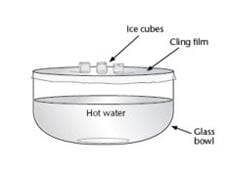
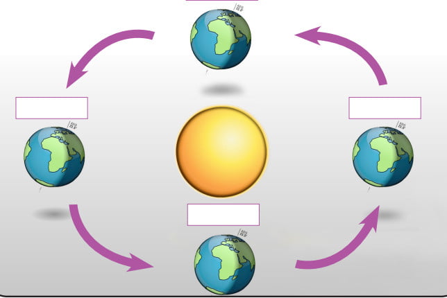


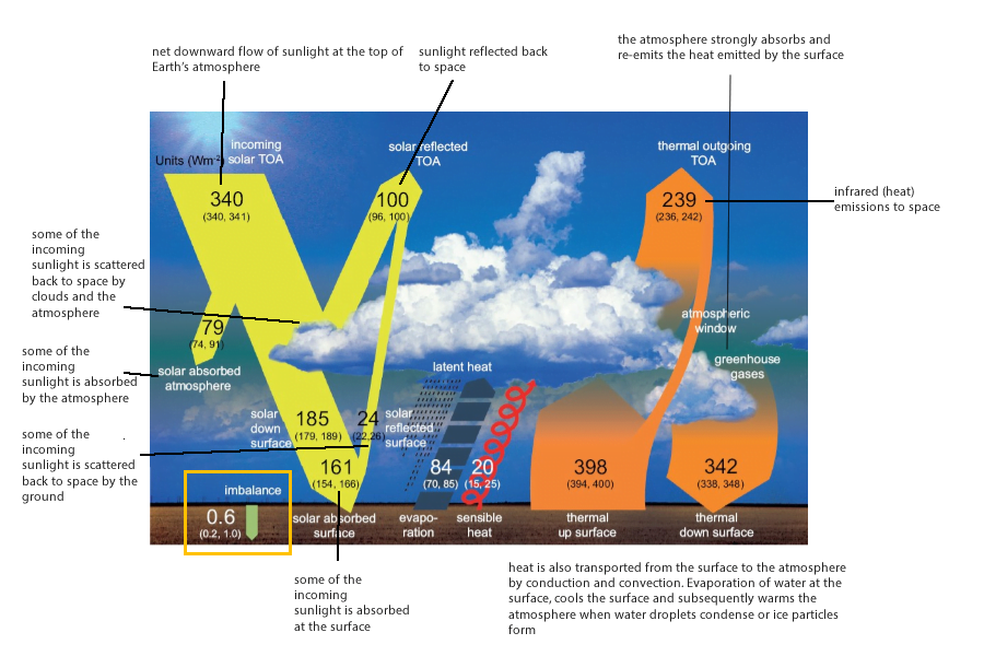
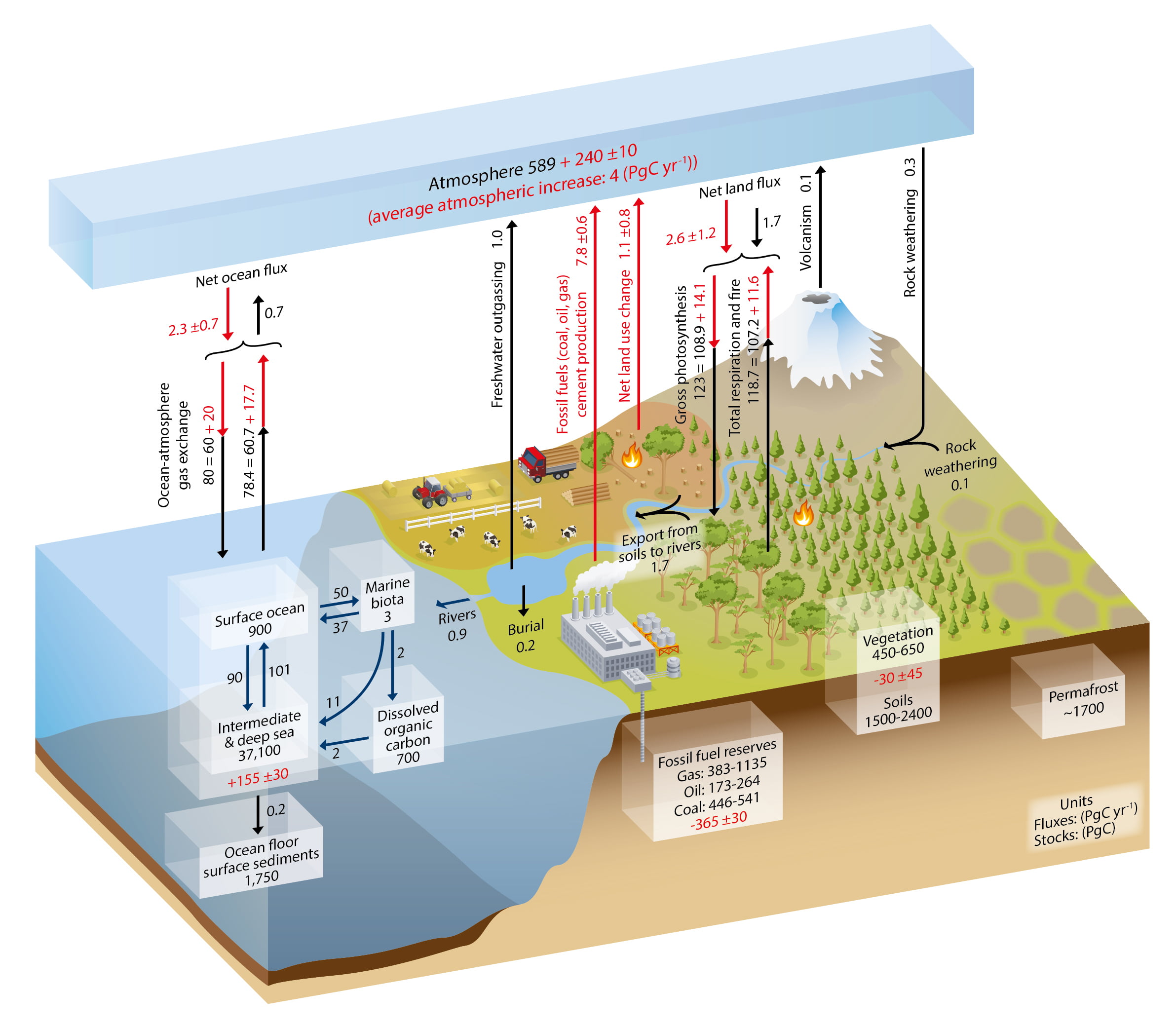
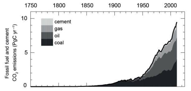
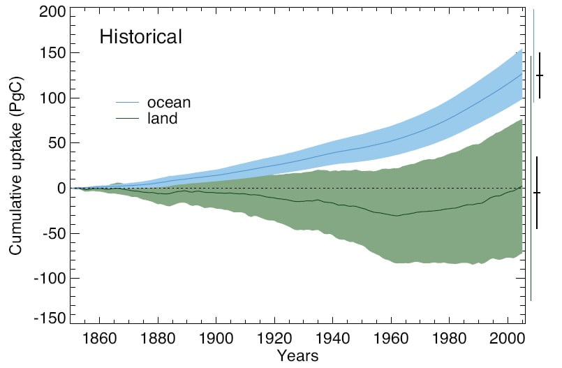
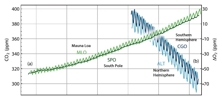

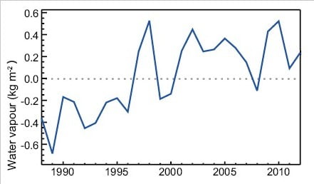
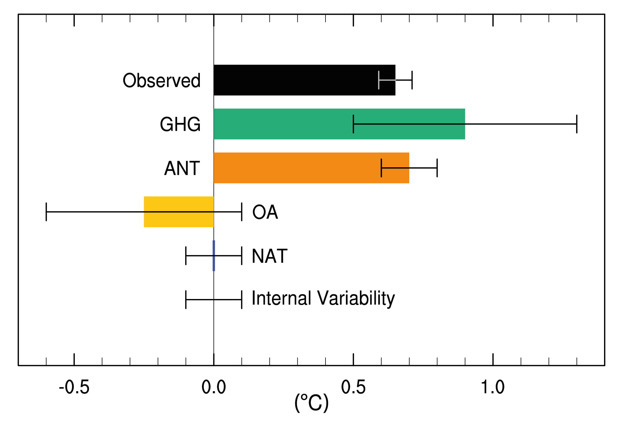

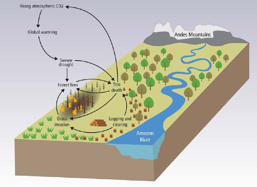


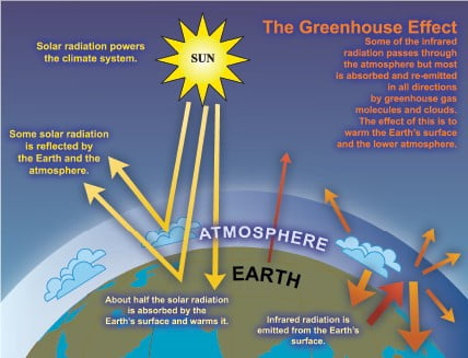


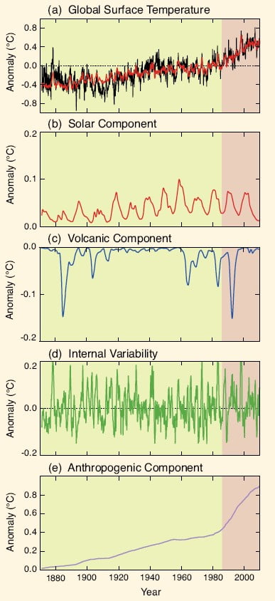

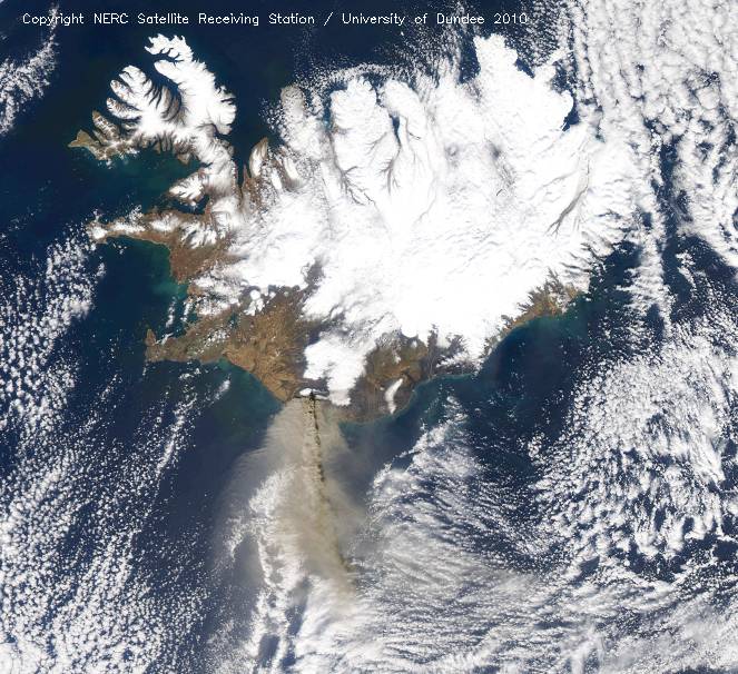
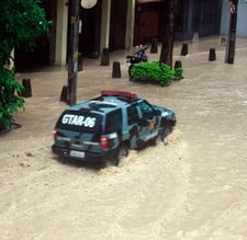

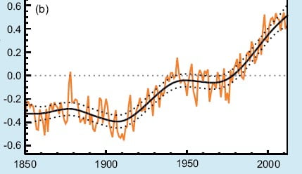
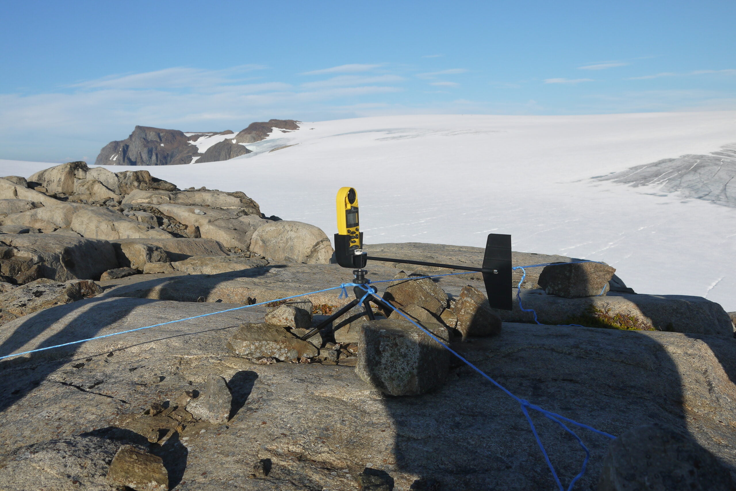

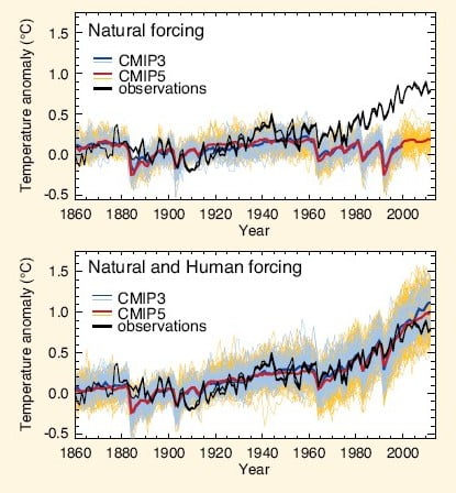

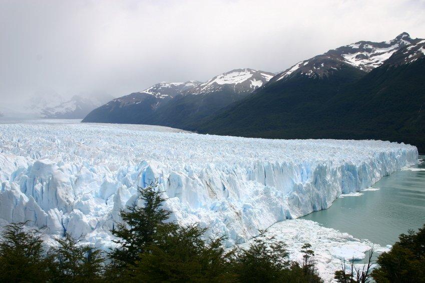


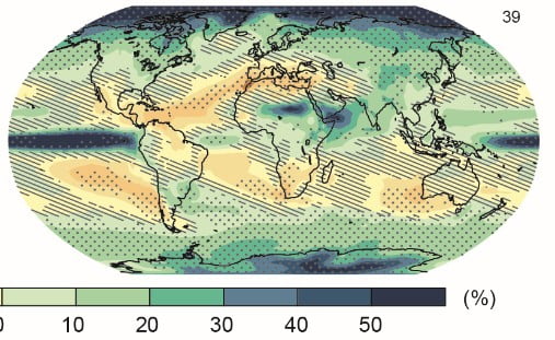
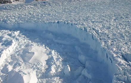
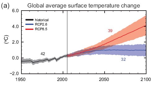
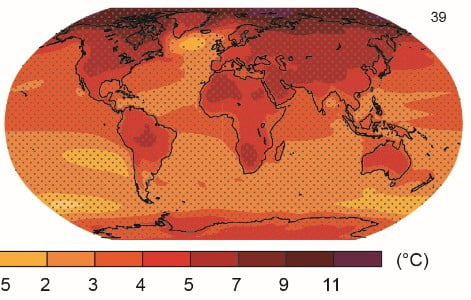
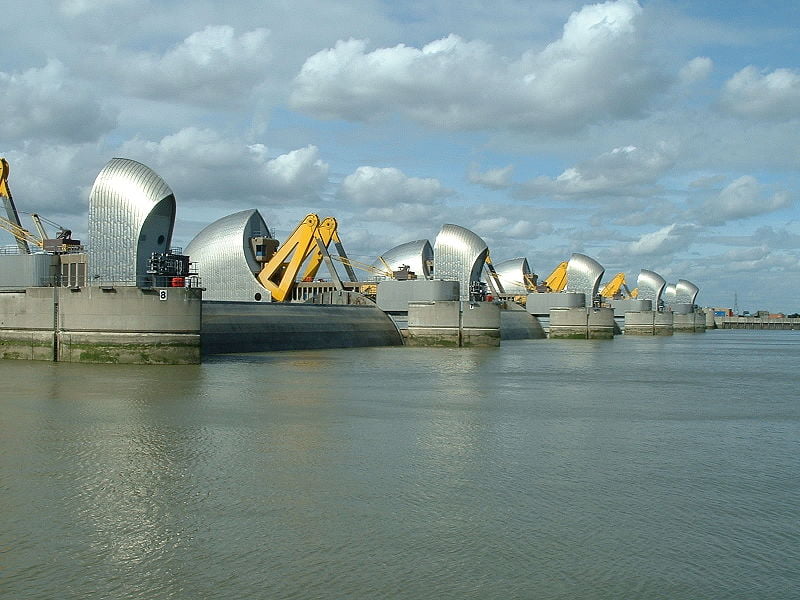
 Storm surges are mainly caused by the effect of the wind on the sea, not changes in atmospheric pressure. The effect of wind on the sea surface is known as wind stress. The wind stress on the surface of the sea causes the water level on a coast to rise if the net transport of water is towards land and to fall if it is away from land.
 Flooding of the Thames on 6th -7th January 1928 highlighted the need to find ways of forecasting storm surges. However, the real push to investigate storm-surges was on 31st January and 1st February 1953, when, a surge exceeding 2.7 metres at Southend in Essex and 3.5 metres in parts of Holland killed 307 people died in eastern England and 1,800 in the Netherlands. The storm that caused the 1953 surge was among the worst to hit the UK in the 20th century. Before the storm’s low pressure and storm-force northerly winds raised water levels in the southern North Sea, hurricane-force winds blew down more trees in Scotland than were normally felled in a year; and a car ferry, the Princess Victoria, on passage from Stranraer in Scotland to Larne in Northern Ireland, sank with the loss of 133 lives. Only 41 of the passengers and crew survived. Nowadays, surges are forecast with considerable accuracy and storm-surge barriers are in place in the most vulnerable places in the Low Countries and eastern England, one of them on the Thames a (south of Greenwich).
 When pressure falls by one millibar, sea level rises by one centimetre. Thus, a deep depression can cause sea level to rise 60 or 70cm above the level predicted purely on the basis of tidal theory. The pressure-induced rise in sea level caused by a tropical cyclone can be much greater, maybe a metre or more.
 One of the most energetic and destructive of all weather systems are tropical cyclones. The hurricane-force winds can reach 50m/s and torrential rain falls from their towering cumulonimbus clouds.flooding The winds can cause disastrous surges on coasts and the downpours of rain can cause serious flooding. Power and water supplies are disrupted, buildings are damaged, crops are destroyed, people and livestock are drowned, bridges collapse, roads and railways are undermined or blocked by debris, and beaches are scoured. Tropical cyclones nearly always leave behind a trail of destruction and misery.
 Flash floods are exceedingly dangerous. When water cannot percolate into the ground, it runs off the surface as it would from impermeable concrete. This is particularly so when the ground is very wet or when baked hard after a hot dry spell. Potholers can be especially at risk, such as on 24 June 1967, when five drowned in Yorkshire. The water which fell in a heavy thunderstorm after a spell of dry weather ran off rapidly into underground streams and caverns at Mossdale. The rise in water levels below ground was too rapid for the potholers to scramble to safety.
 In terms of water flow, the Mississippi is the sixth largest river in the world. Its annual average flow rate is 14,000 cubic metres per second and it discharges into the Gulf of Mexico 580 cubic kilometres of fresh water per year. The greatest flows occur in the period March to May and the least in the period August to October. A large proportion of the United States is drained by this river.
 There was rain, more rain and even more rain in northern California soon after Christmas 1996. From 29 December 1996 to 4 January 1997, depression after depression from the central Pacific brought rain to northern California. As the air was unusually warm, a consequence of the precipitation was that large amounts of snow melted. During the week of the storms, 61 cm of rain was recorded. Significant flooding occurred in northern California and southern Oregon and 43 counties were declared disaster areas. Flooding occurred rapidly because soils became saturated and amounts of snowmelt were large. Flood-control reservoirs could not cope, as their storage capacity was no more than moderate because of near-normal rainfall and run-off prior to the onset of the severe weather. Levee failure occurred on several rivers.
 In many parts of the world, there are serious health risks after disastrous flooding. Mosquitoes, flies and other insects may become more abundant than usual, as the filth, debris and stagnant water left by the floods provide suitable breeding conditions. Consequences may include out-breaks of typhoid, dysentery and encephalitis. Rats and mice displaced from their natural habitats may find conditions to their liking in houses, sheds, barns and other buildings.
 In some parts of the world, snakes also become a problem after flooding, as they, too, are displaced from their natural homes by the water. Quite often, they appear inside houses. However, snakes can be beneficial, as they help to reduce populations of rodents.
 Some of the most fertile land in the world lies beside rivers, the Nile valley being the classic example. For thousands of years, the people of Egypt have relied upon the waters of the Nile to overflow their banks every year, carrying with them fertile silt that makes agriculture possible. The flow of this river is nowadays controlled by means of the Aswan High Dam, an operation that can have its advantages and disadvantages. Salinity levels in the Nile Delta have increased, for example, because the outflow of fresh water from the river is much less now than before the High Dam existed. On the other hand, availability of water from the lake behind the dam, Lake Nasser, has allowed water levels downstream to be maintained in drought years, thus benefiting agriculture when in olden times crop failure and famine might have occurred.
 The Ganges Delta is another place where flooding brings benefits for agriculture. Here, every June to October, the waters of the Ganges, Brahmaputra and other rivers overflow and inundate the countryside. There is, however, no equivalent of the Aswan High Dam to control the waters of the Ganges Delta. Sometimes, crops are destroyed, hamlets ruined and humans and animals drowned.
 The heavy rains brought by tropical cyclones can help revive crops and replenish water supplies. Sometimes, fruit trees have flowered and borne fruit a second time after the passage of a cyclone. Sometimes, floods have flushed away mosquito breeding areas. There is a danger, however, that residual pools of water will, in turn, become mosquito breeding areas.
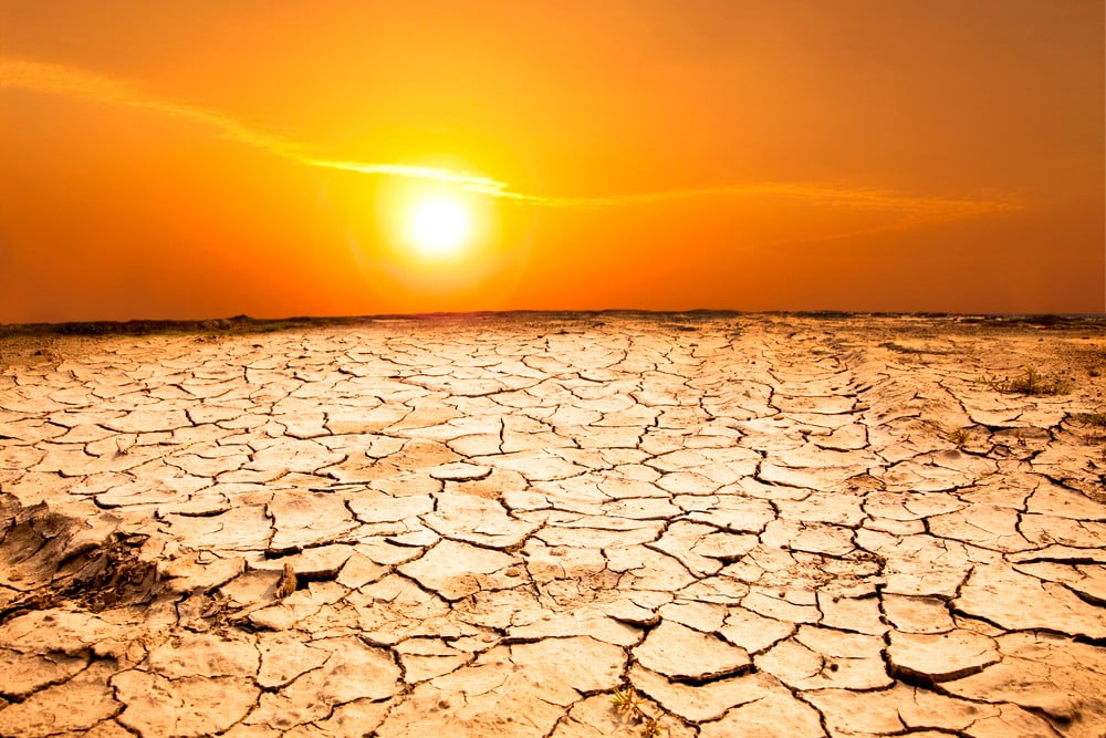
 This is a drought which affects how farmers can use their land. An agricultural drought usually means there is not enough water for the crops to grow as there is a lack of soil moisture. It can also affect livestock such as cows and sheep.
 Hydrological droughts are ones which there is a lack of water at the surface of the earth, resulting in less water in streams, lakes and reservoirs and can impact on the use of water for houses and industry
 This is usually simply defined as a period of time where there has been less rain recorded. Rainfall amounts can vary by duration (i.e. time the rain fell for) and the intensity of rainfall (how hard it was raining). Meteorological drought is usually recorded in the time there has been little or no rain for e.g. months or years.
 A Socioeconomic drought is when physical water shortages affects the lives of people; such as their health and quality of life. It can also affect the supply of food and materials and so affect the economy.


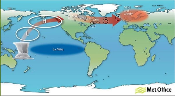

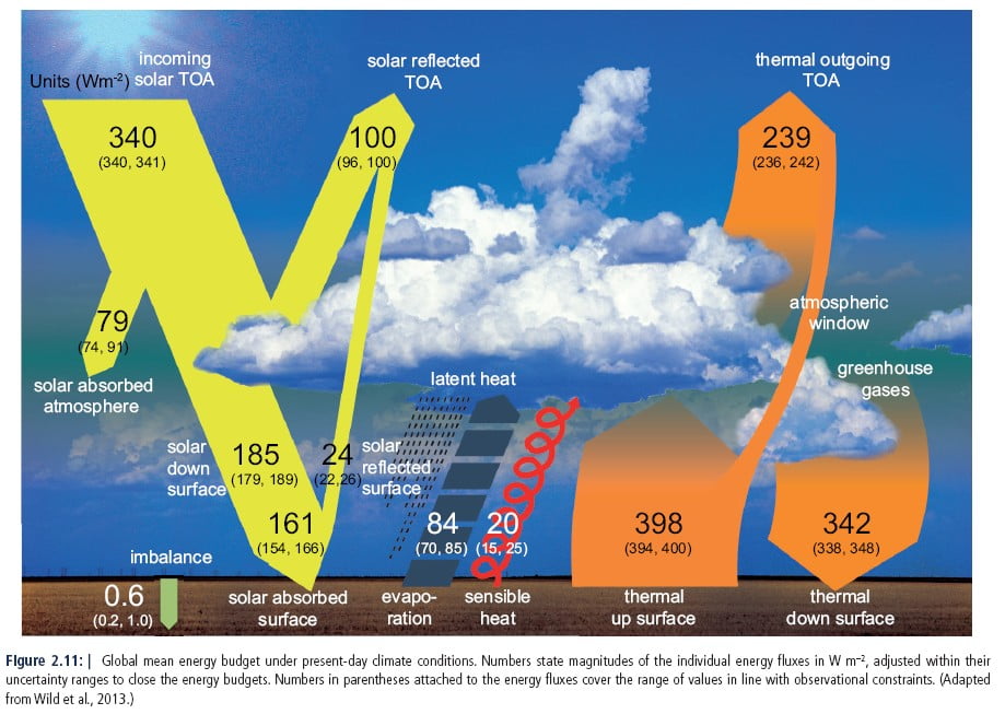
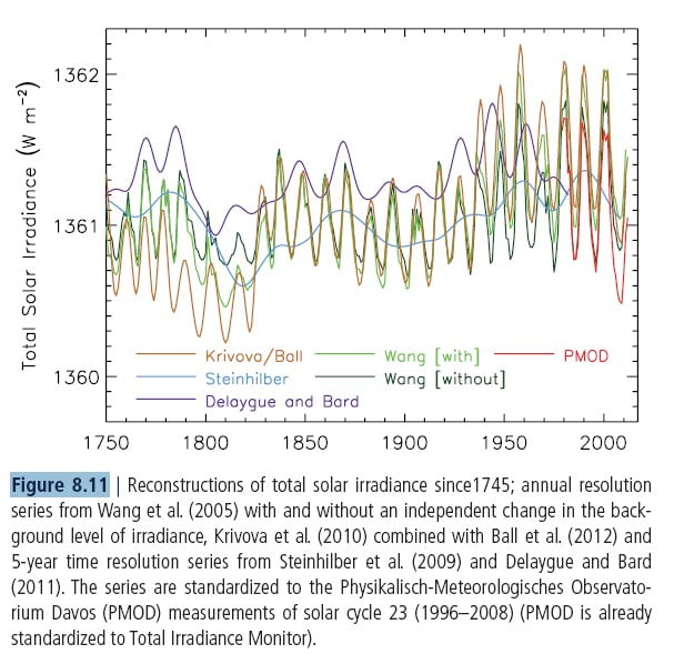
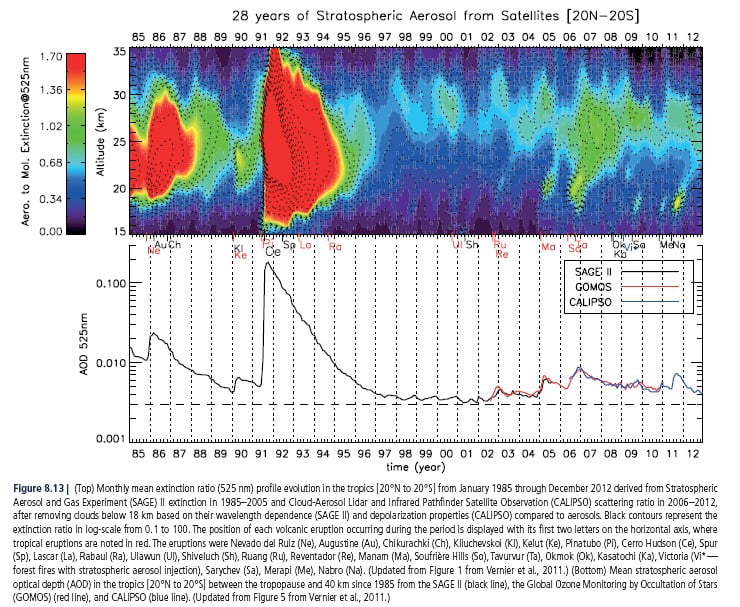
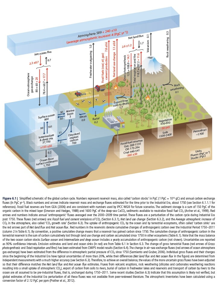
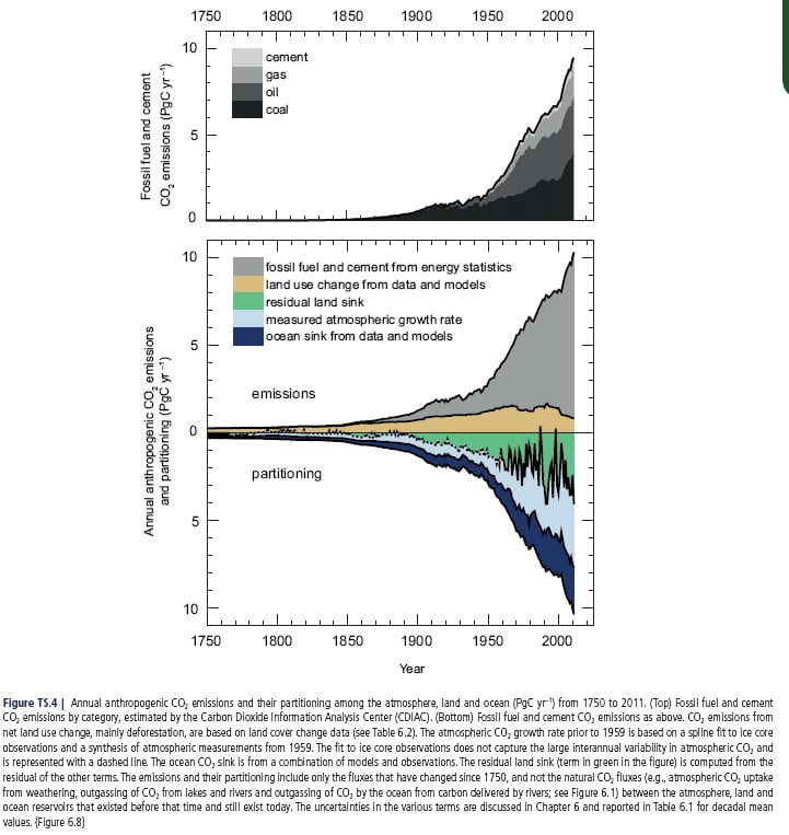
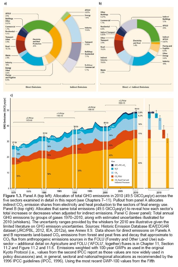
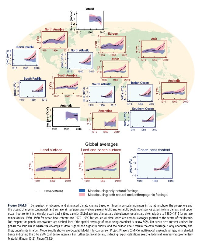
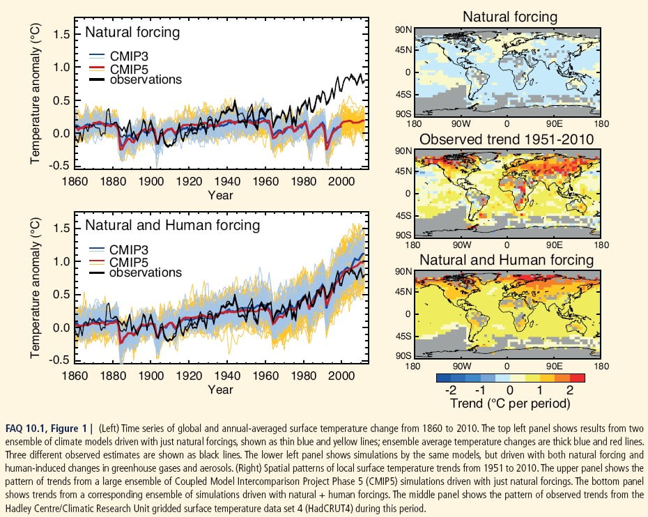
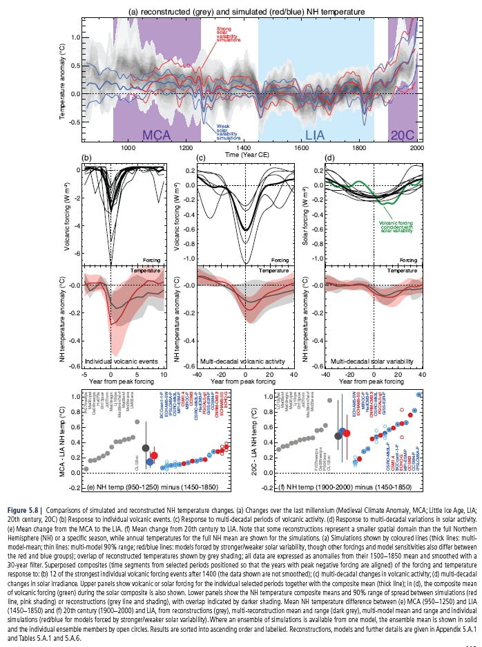
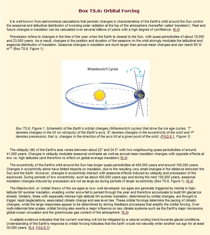
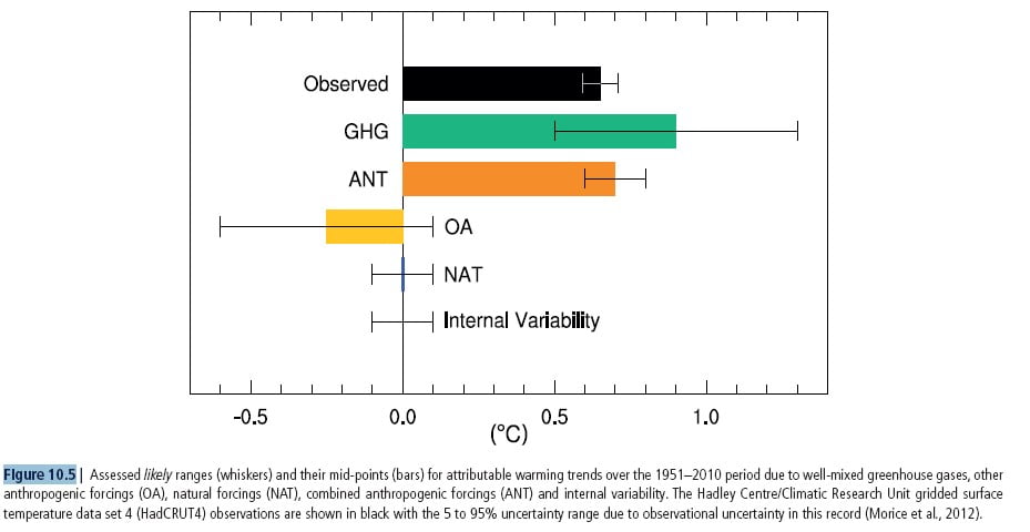
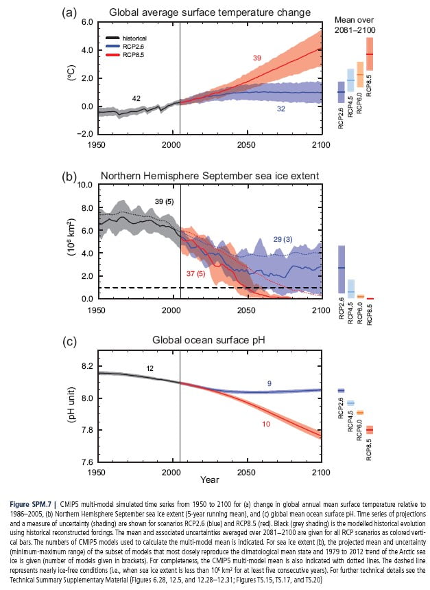
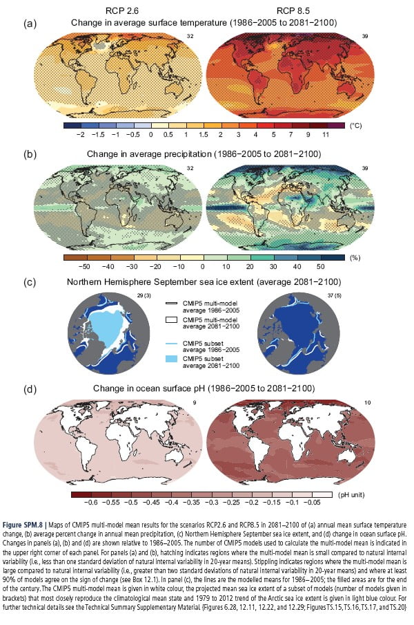
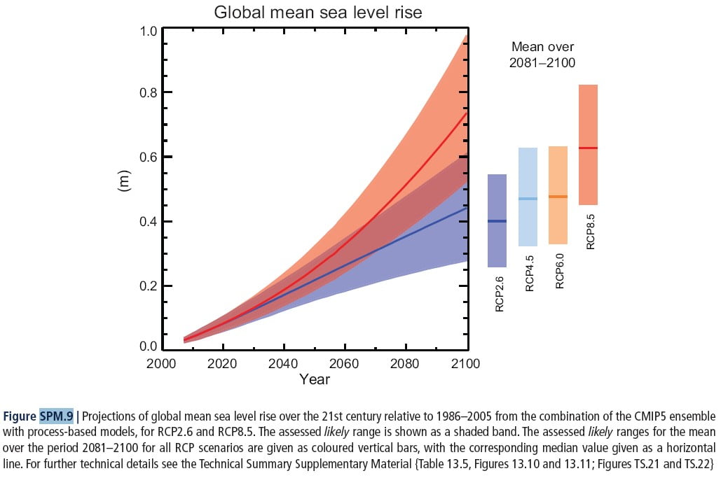
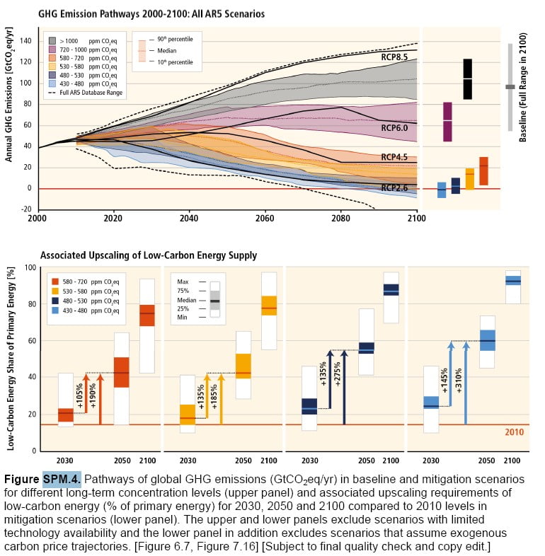
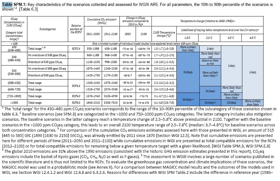
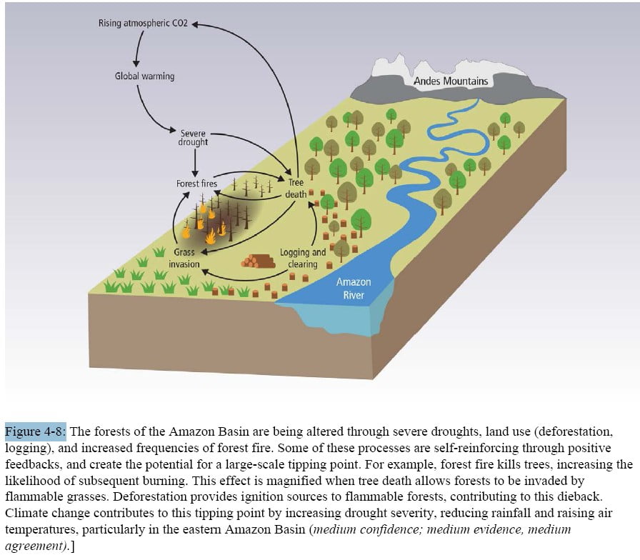
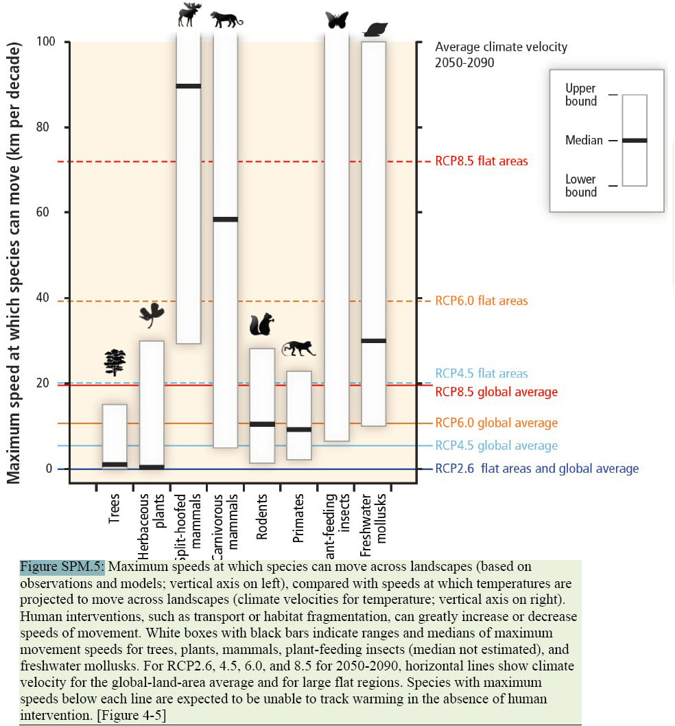
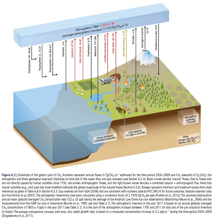
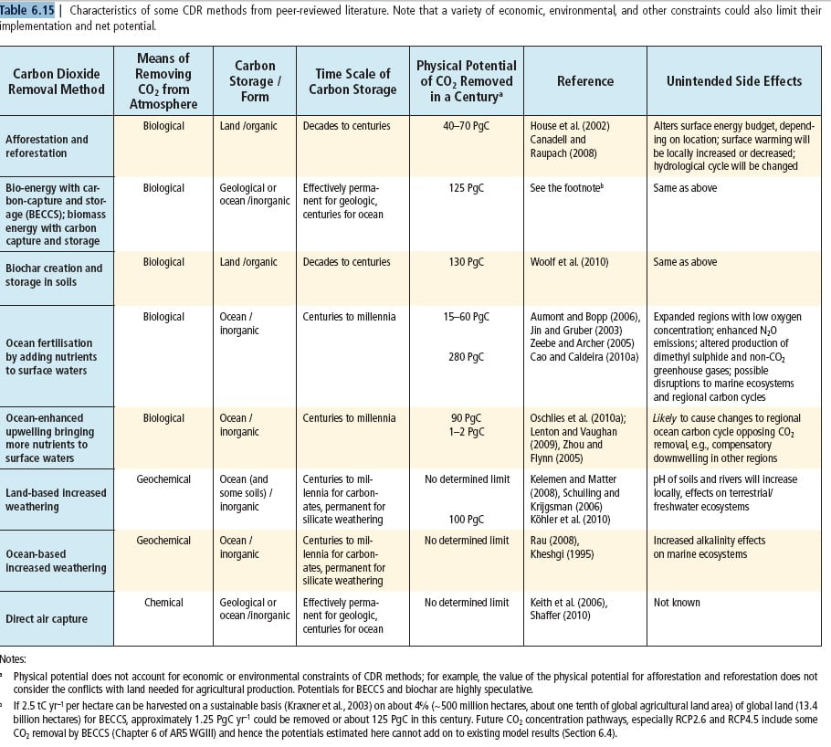