Country-by-Country Emissions of Greenhouse Gases

Questions to consider: Describe the global distribution of carbon emissions
Explain the reasons for the high proportion of global carbon dioxide emissions for one country shown on the carbon emissions map.

PDF Download

emissions map
Carbon Emissions Map, resizing the territories according to their proportion of global carbon dioxide emissions and colouring them according to their per capita emissions. Reproduced with permission from Dr. Benjamin Hennig http://www.viewsoftheworld.net/ .

Summary:

  • The increase in CO2 emissions from both fossil fuel burning and land use change are the dominant cause of the observed increase in atmospheric CO2 concentration, which is now over 40% above pre-industrial levels.
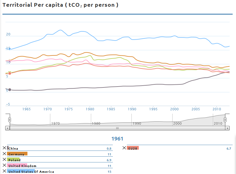
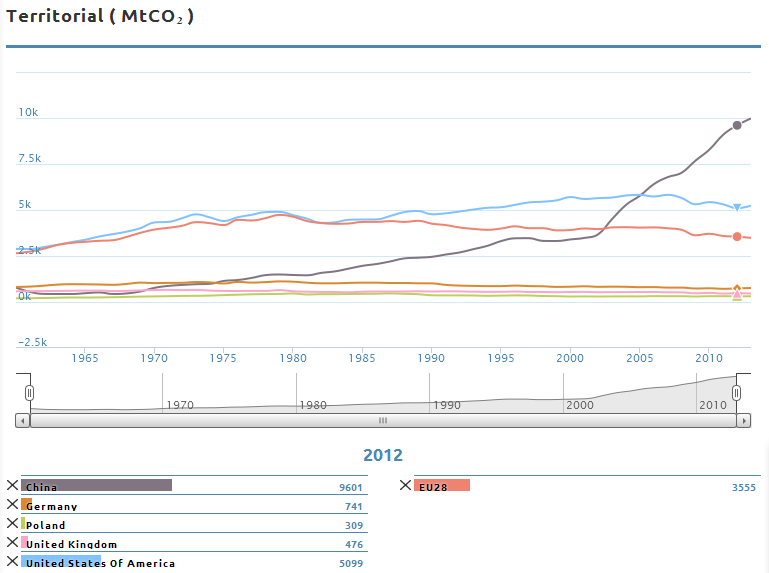
  • Global CO2 emissions have continued to grow over the last 10 years, but there are large variations in emission trajectories between countries.
  • The Ocean has absorbed about 30% of the emitted anthropogenic carbon dioxide.
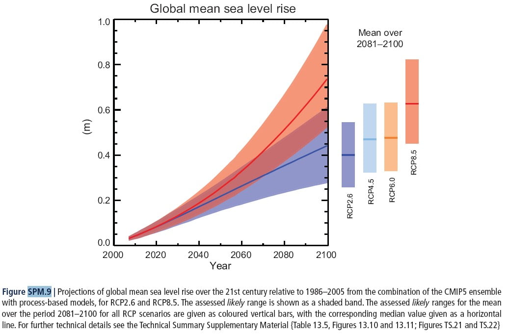
  • Anthropogenic CO2 emissions are currently closest to the highest emissions scenario the IPCC considered.

Case Studies

Reducing greenhouse gas emissions in Germany, an Advanced Country (AC)

Reducing greenhouse gas emissions in the USA, an Advanced Country (AC)

Reducing greenhouse gas emissions in China, an Emerging and Developing Country (EDC)

Reducing greenhouse gas emissions in Poland, an Emerging and Developing Country (EDC)

Return to IPCC updates for A level geography

Further Information

Figure reproduced with permission from the Global Carbon Atlas: globalcarbonatlas.org
Data sources CDIAC: Boden, TA, G Marland, and RJ Andres. 2013. Global, Regional, and National Fossil-Fuel CO2 Emissions. Carbon Dioxide Information Analysis Center (CDIAC), Oak Ridge National Laboratory, US Department of Energy, Oak Ridge, Tenn., USA doi:10.3334/CDIAC/00001_V2013 http://cdiac.ornl.gov/trends/emis/meth_reg.html and UN: United Nations Population Division – World Population Prospects: The 2012 Revision, 2013 http://esa.un.org/unpd/wpp/Excel-Data/population.htm

What Happens to Carbon Dioxide After It Is Emitted into the Atmosphere?
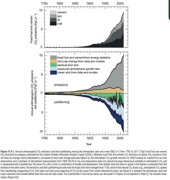
WG1 Chapter 6, Figure 8.
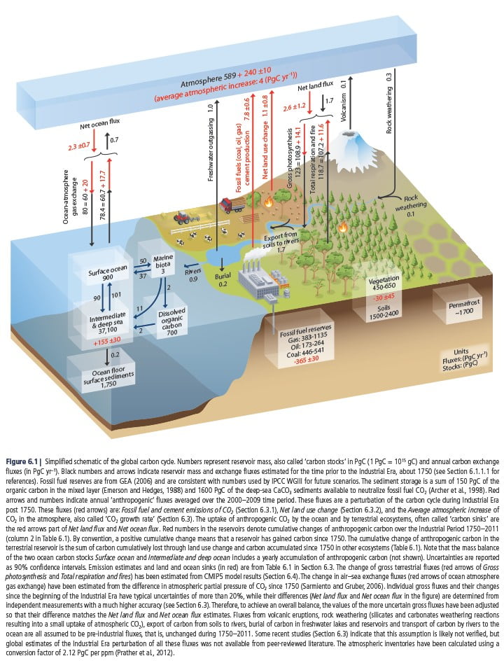
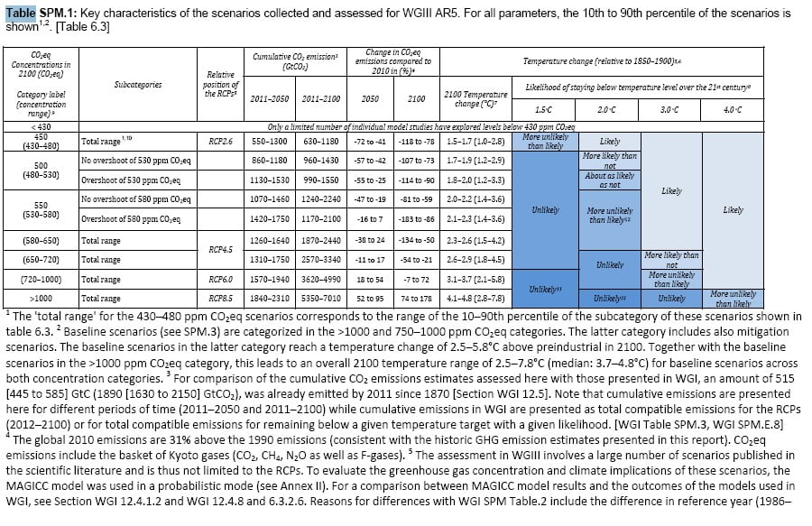
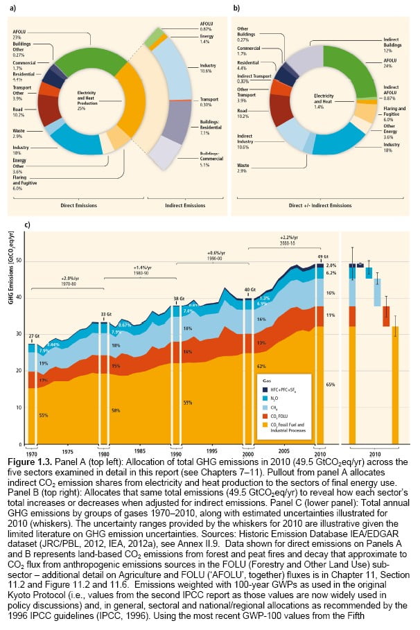
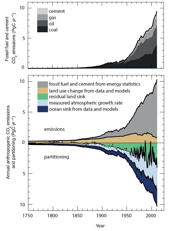
Annual anthropogenic CO2 emissions and their partitioning among the atmosphere, land and ocean (PgC yr–1) from 1750 to 2011. (Top) Fossil fuel and cement CO2 emissions by category (Bottom) Fossil fuel and cement CO2 emissions, CO2 emissions from net land use change (mainly deforestation), the atmospheric CO2 growth rate, the ocean CO2 sink  and the residual land sink which represents the sink of anthropogenic CO2 in natural land ecosystems. The emissions and their partitioning only include the fluxes that have changed since 1750, and not the natural CO2 fluxes (e.g., atmospheric CO2 uptake from weathering, outgassing of CO2 from lakes and rivers, and outgassing of CO2 by the ocean from carbon delivered by rivers) between the atmosphere, land and ocean reservoirs that existed before that time and still exist today. WG1 Chapter 6, Figure 8.

Anthropogenic CO2 emissions to the atmosphere were 555 ± 85 PgC between 1750 and 2011. Of this, fossil fuel combustion and cement production contributed 375 ± 30 PgC and land use change (including deforestation, afforestation (planting new forest) and reforestation) contributed 180 ± 80 PgC. In 2002–2011, average fossil fuel and cement manufacturing emissions were 7.6 to 9.0 PgC/ year, with an average increase of 3.2%/ year compared with 1.0%/ year during the 1990s. In 2011, fossil fuel emissions were in the range of 8.7 to 10.3 PgC.

Emissions due to land use changes between 2002 and 2011 are dominated by tropical deforestation, and are estimated to range between 0.1 to 1.7 PgC/year. This includes emissions from deforestation of around 3 PgC/ year compensated by an uptake of around 2 PgC/year by forest regrowth (mainly on abandoned agricultural land).
The IPCC concluded that the increase in CO2 emissions from both fossil fuel burning and land use change are the dominant cause of the observed increase in atmospheric CO2 concentration.

Reducing greenhouse gas emissions in Germany, an Advanced Country (AC)

Between 1990 and 2014, most major German sources of emissions achieved CO2 reductions. In the energy industry sector, which is responsible for the largest share (around 40%) of Germany’s greenhouse gas emissions, emissions fell by 24% between 1990 and 2014. Even bigger reductions were achieved by households (32.9 %) and industry (33.8 %), helped by the fall of the Berlin wall and the subsequent decline of East German industry and power production and the 2009 economic crisis. The transport sector only reduced its emissions by 0.2 %.
Around half of German electricity is still produced in coal- and gas-fired power plants but Germany is pushing ahead with its transition to renewable energy sources. The production costs of renewable energy have dropped by 70% in the past 5 years, making them a much more competitive energy source. In 2015 the share of renewables in the country’s domestic energy mix increased to 33%,
At the same time, Germany managed to cut down its power consumption in the past year by 3.8%, despite a booming economy (+1.4 %) which generally translates into a higher energy demand, by using LED technology and energy saving measures. CO2 emissions correspondingly fell by 5%. However, 4% of that figure is linked to mild weather conditions requiring less heating.
In 2011, Germany took 8 nuclear power plants off the grid after the Fukushima disaster.
Germany aims to cut greenhouse gas emissions by 40% by 2020 and up to 95% in 2050. It may struggle to meet those targets.
Additional Sources: https://www.cleanenergywire.org/factsheets/germanys-greenhouse-gas-emissions-and-climate-targets , http://www.dw.com/en/renewables-help-cut-german-co2-emissions/a-18176835

https://data.worldbank.org/indicator/EN.ATM.CO2E.PC?locations=DE

Reducing greenhouse gas emissions in the USA, an Advanced Country (AC)

Until 2006, when it was overtaken by China, the USA was the largest emitter of greenhouse gases.
The largest contributor to U.S. greenhouse gas emissions is carbon dioxide from fossil fuel combustion. Changes in this are influenced by many long-term and short-term factors, including population and economic growth, energy price fluctuations, technological changes and the mix of fuels used for electricity generation, short term economic conditions and the weather.
U.S. emissions increased by 5.9 % from 1990 to 2013.
From 2010 to 2011, CO2 emissions from fossil fuel combustion decreased by 2.5 % due to:
(1) a decrease in coal consumption, with increased natural gas consumption and a significant increase in hydropower used;
(2) a decrease in transportation-related energy consumption due to higher fuel costs, improvements in fuel efficiency, and a reduction in miles travelled; and
(3) relatively mild winter conditions resulting in an overall decrease in energy demand in most sectors.
From 2011 to 2012, CO2 emissions from fossil fuel combustion decreased by 3.9 %, with emissions from fossil fuel combustion at their lowest level since 1994 due to:

(1) a slight increase in the price of coal, and a significant decrease in the price of natural gas;
(2) the weather conditions, with no extremely hot days in the summer and much warmer than usual winter temperatures leading to heating degree days decreasing by 12.6 %. This decrease in heating degree days resulted in a decreased demand for heating fuel in the residential and commercial sector, which had a decrease in natural gas consumption of 11.7 and 8.0 %, respectively.

From 2012 to 2013, CO2 emissions from fossil fuel combustion increased by 2.6 % due to:
(1) the weather – heating degree days increased 18.5 % in 2013 compared to 2012.
(2)The consumption of natural gas used to generate electricity decreased by 10.2 % due to an increase in the price of natural gas. Electric power plants shifted some consumption from natural gas to coal, increasing coal consumption to generate electricity by 4.2 %.

The use of fracking to extract natural gas is expected to reduce American emissions in the future, by reducing its reliance on coal.

Additional Sources:
http://www3.epa.gov/climatechange/science/indicators/ghg/us-ghg-emissions.html
http://www3.epa.gov/climatechange/ghgemissions/usinventoryreport.html
http://www3.epa.gov/climatechange/Downloads/ghgemissions/US-GHG-Inventory-2014-Chapter-2-Trends.pdf
http://climateactiontracker.org/countries/usa.html

https://data.worldbank.org/indicator/EN.ATM.CO2E.PC?locations=US

Reducing greenhouse gas emissions in China, an Emerging and Developing Country (EDC

Source: Wikipedia https://en.wikipedia.org/wiki/Economic_history_of_China_(1949–present) Scatter graph of the People’s Republic of China’s GDP between 1952 to 2005, based on publicly available nominal GDP data published by the People’s Republic of China and compiled by Hitotsubashi University (Japan) and confirmed by economic indicator statistics from the World Bank.

China’s emissions started to climb in the 1950s as its economy grew – at an average rate of 10% per year during the period 1990–2004. Over the past 20 years huge numbers of mainly coal fired power stations have been constructed.  In 2003, following legislation to protect private property rights, construction boomed and current rates of housing construction are equivalent to building a city the size of Rome in 2 weeks! China’s total emissions overtook those of the USA in 2006 and its emissions per head of population overtook those of the EU in 2014.
In China, manufacturing and construction account for two thirds of emissions by source (one third of that is steel production, a quarter is cement, chemicals and plastics produce 17%, aluminium and other metals a further 13%) .Unlike most countries, household efficiency is relatively unimportant but sustainable industry is a big priority. It is worth noting that about 20% of Chinese emissions arise from producing clothes, furniture and even solar panels that are shipped to Europe and America.

In the first third of 2015, China dramatically cut its carbon dioxide emissions, with its reduction equalling the UK’s total emissions for the same period. This is largely due to the closure of more than 1,000 coal mines; coal output is down 7.4% year on year. By 2020, China hopes to reduce coal from around 66% of its energy consumption to 62% which should also improve air quality.

China will aim to cut its greenhouse gas emissions per unit of gross domestic product by 60-65% from 2005 levels under a plan submitted to the United Nations for the 2015 COP21 meeting in Paris. China said it would increase the share of non-fossil fuels (wind and solar) as part of its primary energy consumption to about 20% by 2030, and peak emissions by around the same point, though it would “work hard” to do so earlier. Indeed, China is now the world’s largest investor in renewable sources of energy. 

Additional Source: http://climateactiontracker.org/countries/china.html

https://data.worldbank.org/indicator/EN.ATM.CO2E.PC?locations=CN

Reducing greenhouse gas emissions in Poland, an Emerging and Developing Country (EDC)

Poland is not among the largest emitters of greenhouse gases globally (its share is just 1%), but its economy is among the least carbon-efficient in the EU. Among transition economies, Poland’s performance appears better: its carbon intensity on a per capita basis is situated in about the middle of the countries of Eastern and Central Europe and Central Asia. In 2007, around 1.3 metric tonnes of CO2eq, 1.3tCO2eq, were required to produce €1 million in GDP, while the EU average was less than 0.5 tC02eq.

Poland cut its emissions considerably as a side effect of the transition to a market economy, greenhouse gas emissions collapsed along with output through the 90s (declining 20%), as inefficient, often highly energy-intensive plants shut down during the early years of transition.
The period of 1996 to 2002 witnessed another 17 % decline in emissions despite GDP increasing. Overall, although Poland’s GDP nearly doubled from 1988 to 2008, its GHG emissions were reduced by about 30%. During the last half decade or so, a more traditional positive correlation between GDP growth and GHG emissions has re-established itself.

Poland depends on domestically available coal far more than other EU countries (solid fuels, coal and lignite, constitute 57% of gross inland energy consumption for heat and electricity) with very little renewable energy production and no nuclear power. This reliance on coal makes future emission reduction challenging.

Transport, which contributes about 10% of overall GHG emissions, has grown by almost three-quarters since transition, with a very high share of used vehicles, which tend to be much more fuel inefficient and polluting. However, Poland still has relatively low rates of motorisation, suggesting that the growth of road transport could be high in the future.
Poland has made considerable advances in energy efficiency in the past 20 years; yet further efforts are required to bring it to Western European standards.

In 2014, the EU pledged a 40% reduction in greenhouse gas emissions by 2030. To help some countries achieve this, concessions including carbon credits and emissions allowances were made. Poland claimed 60% of the concessions available to 2019, which it will be able to sell to other EU countries, on the condition that it spends the proceeds on diversifying its energy mix and modernising its coal fired power stations.

Additional Sources:
https://data.worldbank.org/indicator/EN.ATM.CO2E.PC?locations=PL

http://www.oecd.org/newsroom/poland-needs-a-strategy-for-moving-to-a-lower-carbon-economy.htm

national centre for Atmospheric Science logo
RMets logo
Royal Geographical Society Logo

Carbon Cycle Feedbacks

Question to consider:
Outline the significance of permafrost in the carbon cycle.
Explain what is meant by a positive feedback mechanism, using the example of when permafrost thaws.

PDF Download

WG1 Chapter 6, Figure 22.
Maps of the changes in carbon uptake in kg of Carbon/ m2 for:
a) each ppm increase in atmospheric CO2. Orange and red colours indicate that, as the amount of carbon dioxide in the atmosphere increases, more carbon is taken up, whereas blue colours show where extra carbon is released.
b) each degree Celsius increase in temperature.  Orange and red colours indicate that, as the temperature rises, more carbon is taken up, whereas blue colours show where extra carbon is released. The graphs on the right show the mean carbon uptake by land and ocean for each latitude line corresponding with the adjacent maps. WG1 Chapter 6, Figure 22.

As carbon dioxide concentrations in the atmosphere increase:

  • The oceans will take up more CO2 almost everywhere, but particularly in the North Atlantic and Southern Oceans.
  • The take up of CO2 by land areas will increase everywhere, particularly over tropical land and in humid regions where the amount of biomass is high. There is also a relatively large increase over Northern Hemisphere temperate and boreal latitudes, because of the greater land area and large areas of forest.
  • Without this increased uptake of CO2 by the land and ocean, annual increases in atmospheric carbon dioxide concentration would be around double the observed rates

As the atmosphere warms:

  • Tropical ecosystems will store less carbon, as will mid-latitudes.
  • At high latitudes, the amount of carbon stored on land will increase, although this may be offset by the decomposition of carbon in permafrost.
  • As sea-ice melts, more water is exposed and therefore more CO2 can be taken into the water.
  • As water warms, the solubility of CO2 in water decreases and so less is taken up by the oceans.
  • Ocean warming and circulation changes will reduce the rate of carbon uptake in the Southern Ocean and North Atlantic.

Summary:

  • The physical, biogeochemical carbon cycle in the ocean and on land will continue to respond to climate change and rising atmospheric CO2 concentrations during the 21st century.
  • The effects of increasing carbon dioxide in the atmosphere and increasing temperature do not necessarily have the same impact on the carbon cycle.
  • There is high confidence that climate change (temperature change) will partially offset increases in global land and ocean carbon sinks caused by rising atmospheric CO2.
  • Between about 15 to 40% of human-emitted CO2 will remain in the atmosphere longer than 1,000 years

Case Studies

Carbon Release from the Arctic

< Return to IPCC updates for geography

Further Information

Boreal – Tundra Biome Shift

WG1 Chapter 6, Figure 24.
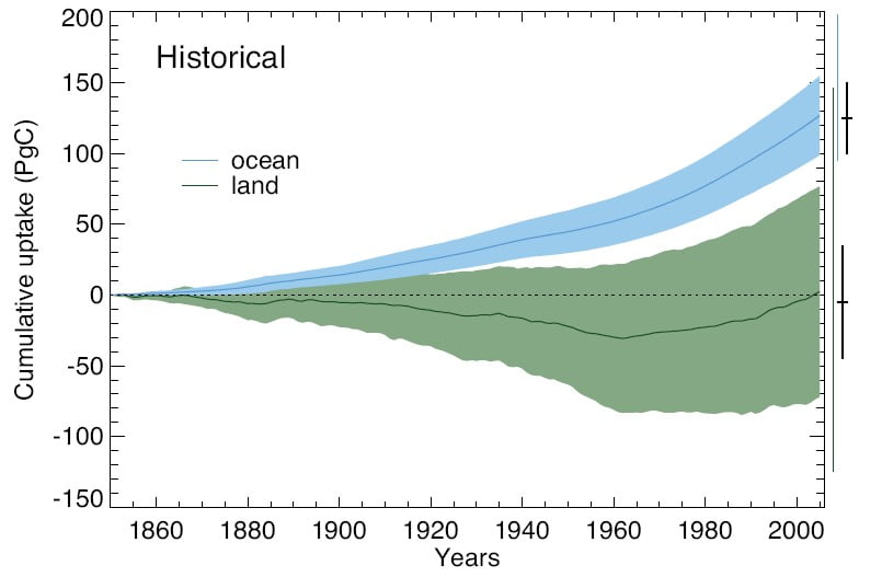
Cumulative land and ocean uptake of carbon for the period 1850-2005. The thick line shows the mean and the shaded area shows one standard deviation. This shows that land was a net source of CO2 to the atmosphere until around 1960, after which land becomes a net sink with more CO2 being drawn down from the atmosphere into vegetation and soils than is released. WG1 Chapter 6, Figure 24.

Boreal – Tundra Biome Shift
WG2 Box 4-4

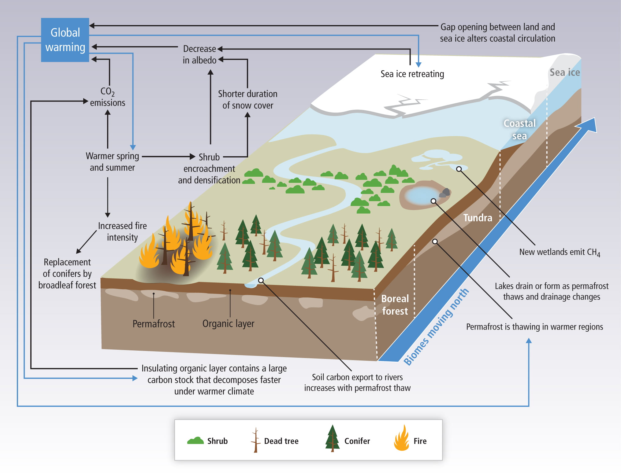
Changes in a suite of ecological processes currently underway across the broader arctic region are consistent with Earth system model predictions of climate-induced geographic shifts in the range extent and functioning of the tundra and boreal forest biomes. Until now, these changes have been gradual shifts across temperature and moisture gradients, rather than abrupt. Responses are expressed through gross and net primary production, microbial respiration, fire and insect disturbance, vegetation composition, species range expansion and contraction, surface energy balance and hydrology, active layer depth and permafrost thaw, and a range of other inter-related variables. Because the high northern latitudes are warming more rapidly than other parts of the Earth, due at least in part to arctic amplification, the rate of change in these ecological processes are sufficiently rapid that they can be documented in situ as well as from satellite observations and captured in Earth system models.

Gradual changes in composition resulting from decreased evergreen conifer productivity and increased mortality, as well as increased deciduous species productivity, can be facilitated by more rapid shifts associated with fire disturbance where it can occur. Each of these interacting processes, as well as insect disturbance and associated tree mortality, are tightly coupled with warming induced drought. Similarly, gradual productivity increases at the boreal-tundra ecotone are facilitated by long distance dispersal into areas disturbed by tundra fire and thermokarsting. In North America these coupled interactions set the stage for changes in ecological processes, already documented, consistent with a biome shift characterized by increased deciduous composition in the interior boreal forest and evergreen conifer migration into tundra areas that are, at the same time, experiencing increased shrub densification. The net feedback of these ecological changes to climate is multi-faceted, complex, and not yet well known across large regions except via modelling studies, which are often poorly constrained by observations.

WG2 Chapter 4, Figure 10.
Tundra-Boreal Biome Shift. Earth system models predict a northward shift of Arctic vegetation with climate warming, as the boreal biome migrates into what is currently tundra. Observations of shrub expansion in tundra, increased tree growth at the tundra-forest transition, and tree mortality at the southern extent of the boreal forest in recent decades are consistent with model projections. Vegetation changes associated with a biome shift, which is facilitated by intensification of the fire regime, will modify surface energy budgets, and net ecosystem carbon balance, permafrost thawing and methane emissions, with net feedbacks to additional climate change. WG2 Chapter 4, Figure 10.

Carbon Release from the Arctic

WG1 Chapter 6, FAQ6.1 Figure 1.

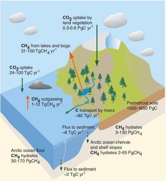
At the moment, vegetation in the Arctic is responsible for about 10% of the CO2 uptake by land globally. Permafrost soils on land and in ocean shelves contain large pools of organic carbon. If permafrost melts, microbes decompose the carbon, releasing it as CO2 or, where oxygen is limited (for example if the soil is covered in standing water), as methane. As the climate of the Arctic warms, more permafrost will thaw. However, warmer Arctic summers would also mean an increase in the amount of vegetation and therefore photosynthesis and CO2 uptake in the Arctic. As yet, scientists don’t know which process will dominate over the next few decades. To complicate matters further, the microbes decomposing the carbon also release heat, causing further melting – a positive feedback.

Methane hydrates are another form of frozen carbon, found in deeper soils. Changes to the temperature and pressure of permafrost soils (and ocean waters) could lead to methane, a gas with a much stronger greenhouse warming potential than carbon dioxide, being released. However, most of the methane is virtually certain to remain trapped underground and will not reach the atmosphere.

The release of carbon dioxide and methane from the Arctic will provide a positive feedback to climate change which will be more important over longer timescales – millennia and longer. 

As Arctic and sub-Arctic regions warm more than the global average, the increase in temperature could lead to more regular fire damage to vegetation and soils and carbon release. More generally, increased vegetation cover lowers albedo, meaning that more of the sun’s light is absorbed which in turn warms the climate locally (another positive feedback), as well as increasing evapotranspiration and carbon uptake.

national centre for Atmospheric Science logo
RMets logo
Royal Geographical Society Logo

IPCC Updates for A Level Geography

Climate Change Updates

This resource was commended by the Scottish Association of Geography Teachers, 2016.

Evidence from the 2013 Intergovernmental Panel on Climate Change (IPCC) Report: for A level Geography Teachers

Factsheets:

1. The Changing Carbon Cycle

– The ocean’s biological pump

2. The Changing Water Cycle

– Changes to groundwater in Uganda

– The mass budgets of Himalayan glaciers

3. Carbon Cycle Feedbacks

– Carbon release from the Arctic

4. Ecosystem Feedbacks from Carbon and Water Cycle Changes

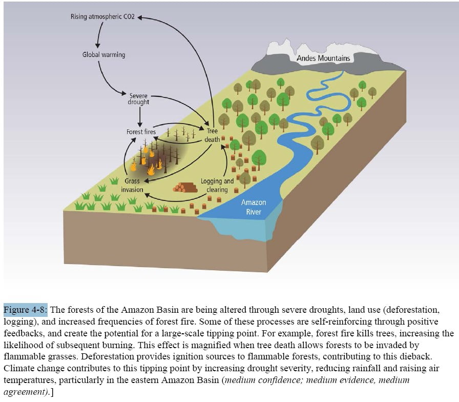
– Vegetation changes in the Amazon Basin

5. Tipping Points: Critical Thresholds for Climate Change

– Summer Arctic sea-ice

6. Impact of Climate Change on Water Supply 

– Water saving irrigation in China
– Upper East Region, Northern Ghana

7. Sea Level Change

– Flood protection in the Netherlands
– Flood protection for London: the Thames barrier

8. Country by Country Emissions of Greenhouse Gases

– Reducing greenhouse gas emissions in China
– Reducing greenhouse gas emissions in Germany
– Reducing greenhouse gas emissions in the USA
– Reducing greenhouse gas emissions in Poland

9. Mitigation Strategies

– The European Union Emissions Trading Scheme
– Developing the Indian solar industry

10. Adaptation Strategies  

– The impact of three urban policies in Paris on climate change adaptation and mitigation

Glossary

Units

Further information about the carbon and water cycles, and wider support for GCSE and A level geography can be downloaded from www.rgs.org/schools.

Unless otherwise stated, the figures, tables and Frequently Asked Questions referenced in this booklet may be downloaded from the IPCC website.

IPCC, 2013: Climate Change 2013: The Physical Science Basis. Working Group I Contribution to the Fifth Assessment Report of the Intergovernmental Panel on Climate Change, Cambridge University Press, Cambridge, United Kingdom and New York, NY, USA.

IPCC, 2014: Climate Change 2014: Impacts, Adaptation and Vulnerability. Working Group II Contribution to the Fifth Assessment Report of the Intergovernmental Panel on Climate Change, Cambridge University Press, Cambridge, United Kingdom and New York, NY, USA.

IPCC, 2014: Climate Change 2014: Mitigation of Climate Change. Working Group III Contribution to the Fifth Assessment Report of the Intergovernmental Panel on Climate Change, Cambridge University Press, Cambridge, United Kingdom and New York, NY, USA.

The Intergovernmental Panel on Climate Change (IPCC) is the leading international body for the assessment of climate change. It was established by the United Nations Environment Programme (UNEP) and the World Meteorological Organization (WMO) in 1988 to provide the world with a clear scientific view on the current state of knowledge in climate change and its potential environmental and socio-economic impacts. It reviews and assesses the most recent scientific, technical and socio-economic information produced worldwide relevant to the understanding of climate change.

RMets logo
national centre for Atmospheric Science logo
Royal Geographical Society Logo

IPCC 2013 Figures

Some Figures and Tables from the IPCC 2013 Fifth Assessment Report

WG1 – The Physical Science Basis

Copyright for all figures:

IPCC, 2013: Climate Change 2013: The Physical Science Basis. Working Group I Contribution to the Fifth Assessment Report of the Intergovernmental Panel on Climate Change, Cambridge University Press, Cambridge, United Kingdom and New York, NY, USA.

WG2- Impacts, Adaptation and Vulnerability

Copyright for all figures:

IPCC, 2014: Climate Change 2014: Impacts, Adaptation, and Vulnerability. Working Group II Contribution to the Fifth Assessment Report of the Intergovernmental Panel on Climate Change, Cambridge University Press, Cambridge, United Kingdom and New York, NY, USA.

WG3 – Mitigation of Climate Change

Copyright for all figures:

IPCC, 2014: Climate Change 2014: Mitigation of Climate Change. Working Group III Contribution to the Fifth Assessment Report of the Intergovernmental Panel on Climate Change, Cambridge University Press, Cambridge, United Kingdom and New York, NY, USA.

In Depth – Climate

Climate

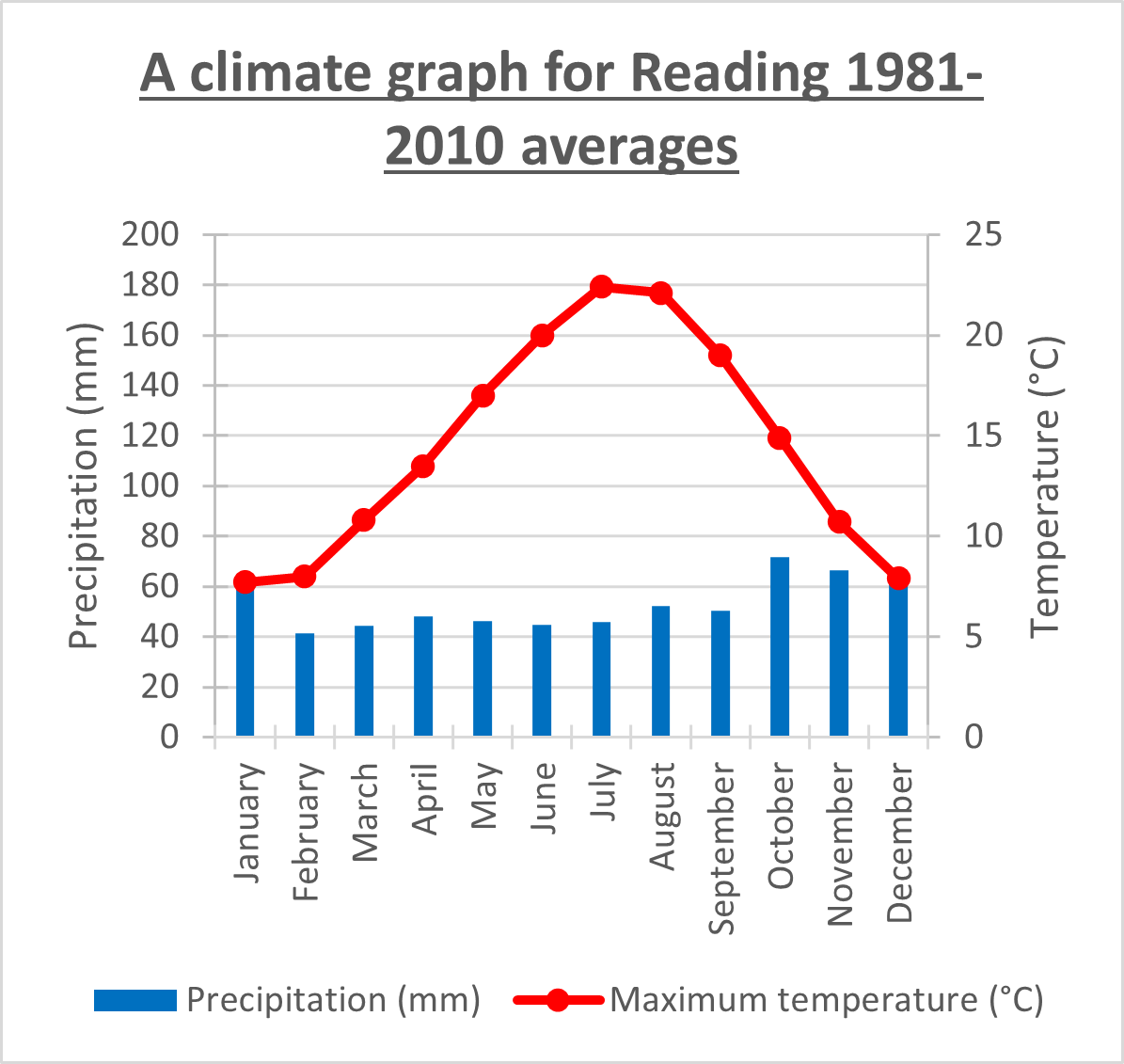
Climate is average weather and its variability over a period of time, ranging from months to millions of years. The World Meteorological Organization standard is a 30-year average.

You can find out more about the climate averages on the Met Office website

Because the atmosphere interacts with the underlying surface – oceans, land, and ice – the term climate system is used to encompass both the atmosphere and the influence of the Earth’s surface on climate.

The climate system consists of five elements: the atmosphere; the ocean; the biosphere; the cryosphere (ice and snow) and the geosphere (rock and soil).

You can find out more about the climate system on the Met Office Site

mountains

World climates

Weather is always changing and the climate in different parts of the world is a combination of all the factors that affect the weather in any particular locality. In some regions of the world there are marked differences between summer and winter climates and here in the UK the climate is very changeable at all times of the year.

Many factors can affect the climate. These include:

  • Distance from the equator
  • Natural features
  • Mountain regions
  • Coastal regions

World climates can be divided into categories

  • Dry
  • Tropical
  • Temperate
  • Cold

Dry
This type of climate is predominantly dry. There are however, three distinct temperature ranges – hot, warm and cold.

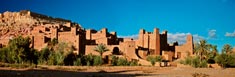
Hot and dry climates are usually desert regions such as the Sahara and the Arabian. These hot deserts have little rain at any season and no real cold weather, although temperature drops sharply at night. Sand or rocks in direct sunlight will easily reach 60 °C to 70 °C (140 °F to 160 °F). But at night temperatures may drop to below freezing.

Warm and dry climates can be found in places that are semi-desert or dry grassland (tropical steppe) such as the Sahel region of Africa or the drier parts of India. In these regions, although there is a rainy season, the rains can fail several years in succession, causing severe drought.

SaharaCold and dry climates can be found in the central parts of Asia, such as the Gobi desert. These cold deserts occur in higher latitudes in the interior of large continents and have a climate that is very hot in summer, but bitterly cold in winter.

Tropical
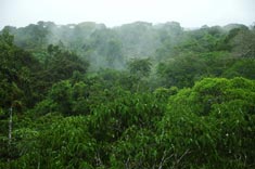
Tropical RainforestMost equatorial and tropical parts of the earth have tropical climates characterised by high temperatures and high humidity throughout the year, and frequent rain throughout most of the year. This region can be split into two distinct types:

  • Tropical wet – there is no distinct wet or dry season, rainfall is distributed throughout the year. This type of climate is characterised by lush tropical forests like the Amazon rain forest, central parts of Africa and Indonesia.
  • Tropical wet and dry – there is a distinction between a wet and dry season. The wet season is usually influenced by monsoon winds that bring large quantities of moisture to a region. Countries like Bangladesh and the eastern side of India have this type of climate.

Temperate
Temperate climate zones lie between the tropics and the polar circles. In these regions the changes between summer and winter are generally subtle – warm or cool rather than extreme; burning hot or freezing cold. However, a temperate climate can have very unpredictable weather. One day it may be sunny, the next it may be raining, and the next it may be cloudy. These erratic weather patterns occur in summer as well as winter.

Temperate climate zones can be split into two distinct types, depending on temperature:

  • Warm temperate – can have rain all year with the wettest weather in summer months, with temperatures ranging from warm to hot all year. Eastern China and the south-eastern states of the USA, such as Florida, are good examples. Mediterranean areas also have a warm wet climate in the winter, but summers tend to be dry with little or no rainfall. Places around the Mediterranean, and some parts of central Chile, California and Western Australia have warm and dry temperate climates ideal for tourism and agriculture.
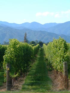
  • New Zealand VinesCold temperate – climates can be wet or dry. Cool and wet climates are places where there is rain every month, but no great extremes of temperature throughout the year. The climates of the British Isles, much of northwest Europe, New Zealand and coastal North America are of this type. The weather can be very changeable and strongly influenced by large moving weather systems called depressions or lows, and anticyclones or highs. Cold and dry climates are places where the weather is dominated by warm summers and cold winters. Regions such as central Europe are of this type.

Cold polar
Cold polar climate is subdivided into Tundra climate and Ice Cap climate. Tundra regions have very short often hot summers followed by bitterly cold and long winters (mean temperature of warmest month between 0 and 10°C). Areas of Canada, northern Russia and Siberia, extending to the Arctic are of this type.

Ice cap or polar climate is characterised by very low temperatures (mean temperature of warmest month below 0 °C), strong winds and year-round snow cover. This type of climate can be found on Greenland and at the Antarctic.

Mountain
Mountain climate can be found in mountainous areas anywhere in the world, where land rises above permanent snowline, generally above 3000m in height. These areas often have cold winters and mild summers. Due to their elevation, temperatures are lower than you would expect for their latitude and the main form of precipitation is snow, often accompanied by strong winds. These areas can be found in the high mountainous areas such as the Andes in South America, the Himalayas and the Tibetan Plateau.

Climate change
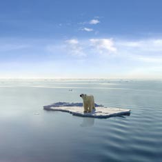
polar bear floating on iceClimate change is a change in the climate’s mean and variability for an extended period of decades, or more.

You can find out more about climate change, climate science and impact from the Met Office


Web page reproduced with the kind permission of the Met Office

How will the UK’s Temperature Change Seasonally (Autumn)?

How will the United Kingdom’s Temperature Change During the 2030’s. 60’s and 90’s? Seasonally – September, October and November

2030
2030
2060
2060
2090
2090
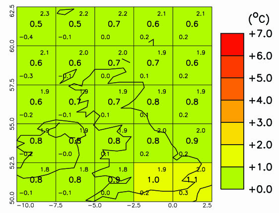
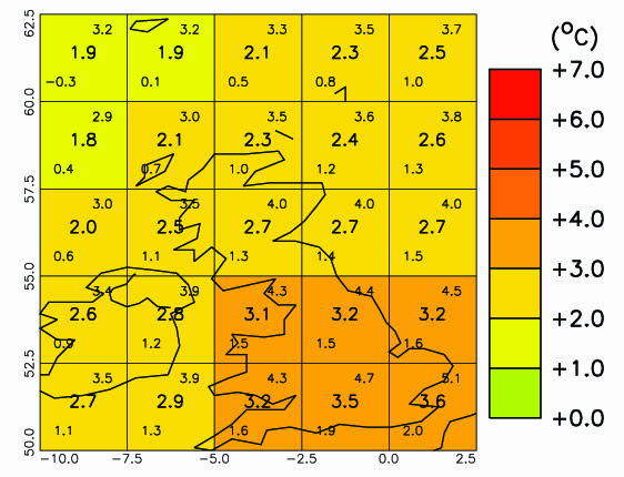
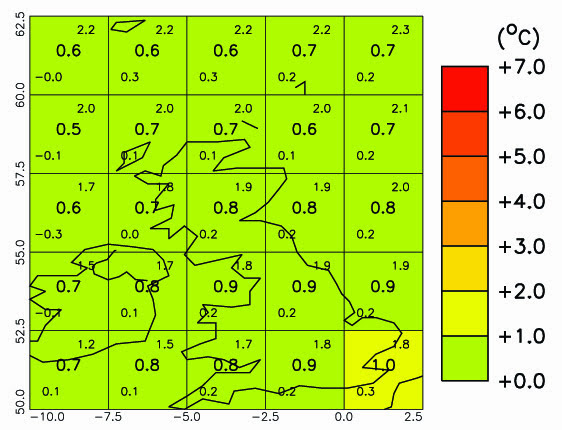
  1. These 3 maps show projected September, October and November (SON) temperatures in the 2030s, 60s and 90s (according to a high carbon dioxide emission scenario, A2).
  2. All values are anomalies – the difference in temperature to the average of 1970 to 1999 temperatures.
  3. Areas shaded red will be 6-7°C hotter than average temperatures from 1970 to 1999, whereas areas shaded green will be about the same as the 1970-1999 average.
  4. The number in the centre of each grid box is the average SON temperature anomaly we expect having had high carbon dioxide emissions; the smaller numbers in the upper and lower corners give the range of average temperature anomalies that might occur.
  5. We use the term SON rather than Autumn because seasons vary around the globe.

McSweeney, C., New, M. and Lizcano, G. (2009) Climate Change Country Profiles – UK. Oxford University School of Geography and Environment and the Tyndall Centre for Climate Change Research. Report commissioned by the British Council, RMetS, RGS-IBG for www.climate4classrooms.org

How will the UK’s Temperature Change Seasonally (Summer)?

June, July, August Temperatures in the 2030’s, 60’s and 90’s

2030
2030
2060
2060
2090
2090
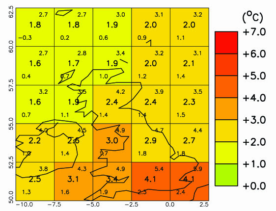
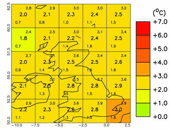
  1. These 3 maps show projected June, July and August (JJA) temperatures in the 2030s, 60s and 90s (according to a high carbon dioxide emission scenario, A2).
  2. All values are anomalies– the difference in temperature to the average of 1970 to 1999 temperatures.
  3. Areas shaded red will be 6-7°C hotter than average temperatures from 1970 to 1999, whereas areas shaded green will be about the same as the 1970-1999 average.
  4. The number in the centre of each grid box is the average JJA temperature anomaly we expect having had high carbon dioxide emissions; the smaller numbers in the upper and lower corners give the range of average temperature anomalies that might occur.
  5. We use the term JJA rather than summer because most climate change maps are for the whole globe and seasons vary around the globe.

McSweeney, C., New, M. and Lizcano, G. (2009) Climate Change Country Profiles – UK. Oxford University School of Geography and Environment and the Tyndall Centre for Climate Change Research. Report commissioned by the British Council, RMetS, RGS-IBG for www.climate4classrooms.org

How will the UK’s Temperature Change Seasonally (Spring)?

How will the UK’s Temperature Change During the 2030’s, 60’s and 90’s? Seasonally – March, April and May.

2030
2030
2060
2060
2090
2090
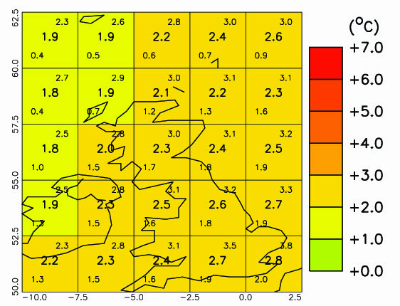
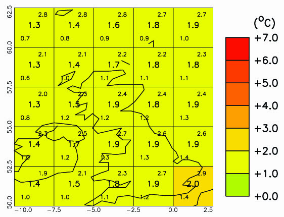
  1. These 3 maps show projected March, April and May (MAM) temperatures in the 2030s, 60s and 90s (according to a high carbon dioxide emission scenario, A2).
  2. All values are anomalies – the difference in temperature to the average of 1970 to 1999 temperatures.
  3. Areas shaded red will be 6-7°C hotter than average temperatures from 1970 to 1999, whereas areas shaded green will be about the same as the 1970-1999 average.
  4. The number in the centre of each grid box is the average MAM temperature anomaly we expect having had high carbon dioxide emissions; the smaller numbers in the upper and lower corners give the range of average temperature anomalies that might occur.
  5. We use the term MAM rather than spring because most climate change maps are for the whole globe and seasons are reversed in the northern and southern hemispheres.

McSweeney, C., New, M. and Lizcano, G. (2009) Climate Change Country Profiles – UK. Oxford University School of Geography and Environment and the Tyndall Centre for Climate Change Research. Report commissioned by the British Council, RMetS, RGS-IBG for www.climate4classrooms.org

How will the UK’s Temperature Change Seasonally – Winter?

How will the UK’s Temperature Change Seasonally – December, January and February

2030
2030
2060
2060
2090
2090
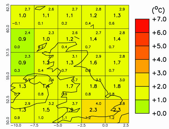
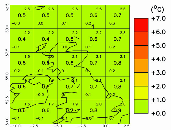
  1. These 3 maps show projected December, January and February (DJF) temperatures in the 2030s, 60s and 90s (according to a high carbon dioxide emissions scenario, A2).
  2. All values are anomalies – the difference in temperature to the average of 1970 to 1999 temperatures.
  3. Areas shaded red will be 6-7°C hotter than average temperatures from 1970 to 1999, whereas areas shaded green will be the same as the 1970-1999 average.
  4. The number in the centre of each grid box is the average projected temperature; numbers in the upper and lower corners give the highest and lowest possible DJF mean temperature.


McSweeney, C., New, M. and Lizcano, G. (2009) Climate Change Country Profiles – UK. Oxford University School of Geography and Environment and the Tyndall Centre for Climate Change Research. Report commissioned by the British Council, RMetS, RGS-IBG for www.climate4classrooms.org

How will the UK’s Temperature Change?

How will the UK’s Temperature Change Between 2009 and 2100

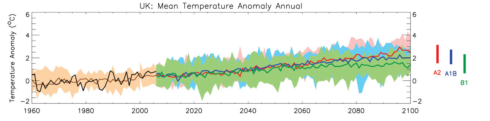
  1. The green, blue and red lines show projected future temperature anomalies from 2006 to 2100, according to three different emission scenarios – green (low), blue (medium) and red (high). The shading around each line shows the range of temperature that might be possible with each emission scenario. The anomaly is the difference in temperature between the year’s projected temperature and the average of all years between 1970 and 1999. If the anomaly is positive, that year was warmer than the 1970-1999 average. If it is negative, that year was colder than the 1970-1999 average.
  2. All scenarios show future temperatures will be warmer.
  3. Average annual temperature is expected to increase by 0.4 to 2.4°Cby the 2060s, and 0.6 to 3.2°C by the 2090s.

McSweeney, C., New, M. and Lizcano, G. (2009) Climate Change Country Profiles – UK. Oxford University School of Geography and Environment and the Tyndall Centre for Climate Change Research. Report commissioned by the British Council, RMetS, RGS-IBG for www.climate4classrooms.org

MetLink - Royal Meteorological Society
We use cookies on this site to enhance your user experienceBy clicking any link on this page you are giving your consent for us to set cookies. More info

By clicking any link on this page you are giving your consent for us to set cookies. More info