Question to consider:
Outline the significance of permafrost in the carbon cycle.
Explain what is meant by a positive feedback mechanism, using the example of when permafrost thaws.

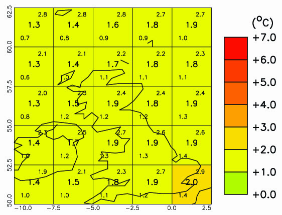
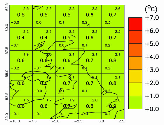
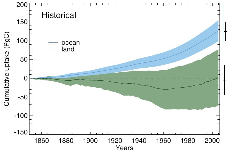
a) each ppm increase in atmospheric CO2. Orange and red colours indicate that, as the amount of carbon dioxide in the atmosphere increases, more carbon is taken up, whereas blue colours show where extra carbon is released.
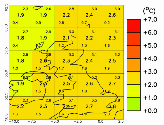
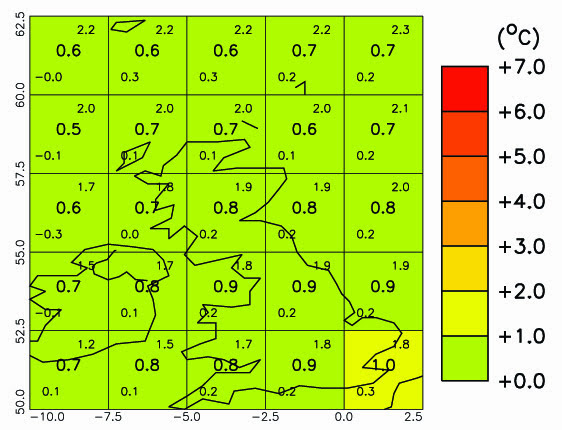
b) each degree Celsius increase in temperature. Orange and red colours indicate that, as the temperature rises, more carbon is taken up, whereas blue colours show where extra carbon is released. The graphs on the right show the mean carbon uptake by land and ocean for each latitude line corresponding with the adjacent maps. WG1 Chapter 6, Figure 22.
As carbon dioxide concentrations in the atmosphere increase:
- The oceans will take up more CO2 almost everywhere, but particularly in the North Atlantic and Southern Oceans.
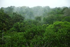
- The take up of CO2 by land areas will increase everywhere, particularly over tropical land and in humid regions where the amount of biomass is high. There is also a relatively large increase over Northern Hemisphere temperate and boreal latitudes, because of the greater land area and large areas of forest.
- Without this increased uptake of CO2 by the land and ocean, annual increases in atmospheric carbon dioxide concentration would be around double the observed rates
As the atmosphere warms:
- Tropical ecosystems will store less carbon, as will mid-latitudes.
- At high latitudes, the amount of carbon stored on land will increase, although this may be offset by the decomposition of carbon in permafrost.
- As sea-ice melts, more water is exposed and therefore more CO2 can be taken into the water.
- As water warms, the solubility of CO2 in water decreases and so less is taken up by the oceans.
- Ocean warming and circulation changes will reduce the rate of carbon uptake in the Southern Ocean and North Atlantic.
Summary:
- The physical, biogeochemical carbon cycle in the ocean and on land will continue to respond to climate change and rising atmospheric CO2 concentrations during the 21st century.
- The effects of increasing carbon dioxide in the atmosphere and increasing temperature do not necessarily have the same impact on the carbon cycle.
- There is high confidence that climate change (temperature change) will partially offset increases in global land and ocean carbon sinks caused by rising atmospheric CO2.
- Between about 15 to 40% of human-emitted CO2 will remain in the atmosphere longer than 1,000 years
Case Studies
Carbon Release from the Arctic
Further Information
Boreal – Tundra Biome Shift
Boreal – Tundra Biome Shift
WG2 Box 4-4
Changes in a suite of ecological processes currently underway across the broader arctic region are consistent with Earth system model predictions of climate-induced geographic shifts in the range extent and functioning of the tundra and boreal forest biomes. Until now, these changes have been gradual shifts across temperature and moisture gradients, rather than abrupt. Responses are expressed through gross and net primary production, microbial respiration, fire and insect disturbance, vegetation composition, species range expansion and contraction, surface energy balance and hydrology, active layer depth and permafrost thaw, and a range of other inter-related variables. Because the high northern latitudes are warming more rapidly than other parts of the Earth, due at least in part to arctic amplification, the rate of change in these ecological processes are sufficiently rapid that they can be documented in situ as well as from satellite observations and captured in Earth system models.
Gradual changes in composition resulting from decreased evergreen conifer productivity and increased mortality, as well as increased deciduous species productivity, can be facilitated by more rapid shifts associated with fire disturbance where it can occur. Each of these interacting processes, as well as insect disturbance and associated tree mortality, are tightly coupled with warming induced drought. Similarly, gradual productivity increases at the boreal-tundra ecotone are facilitated by long distance dispersal into areas disturbed by tundra fire and thermokarsting. In North America these coupled interactions set the stage for changes in ecological processes, already documented, consistent with a biome shift characterized by increased deciduous composition in the interior boreal forest and evergreen conifer migration into tundra areas that are, at the same time, experiencing increased shrub densification. The net feedback of these ecological changes to climate is multi-faceted, complex, and not yet well known across large regions except via modelling studies, which are often poorly constrained by observations.
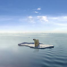
Carbon Release from the Arctic
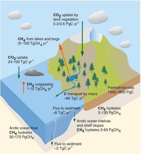
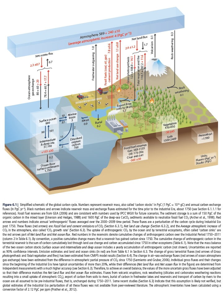
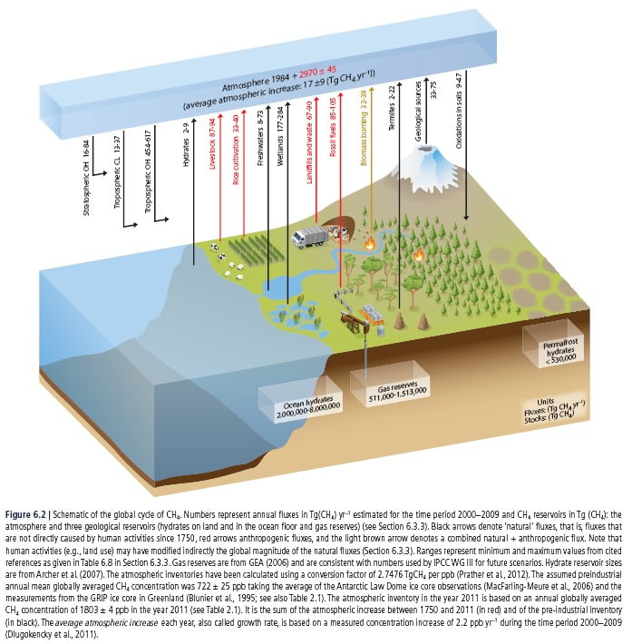
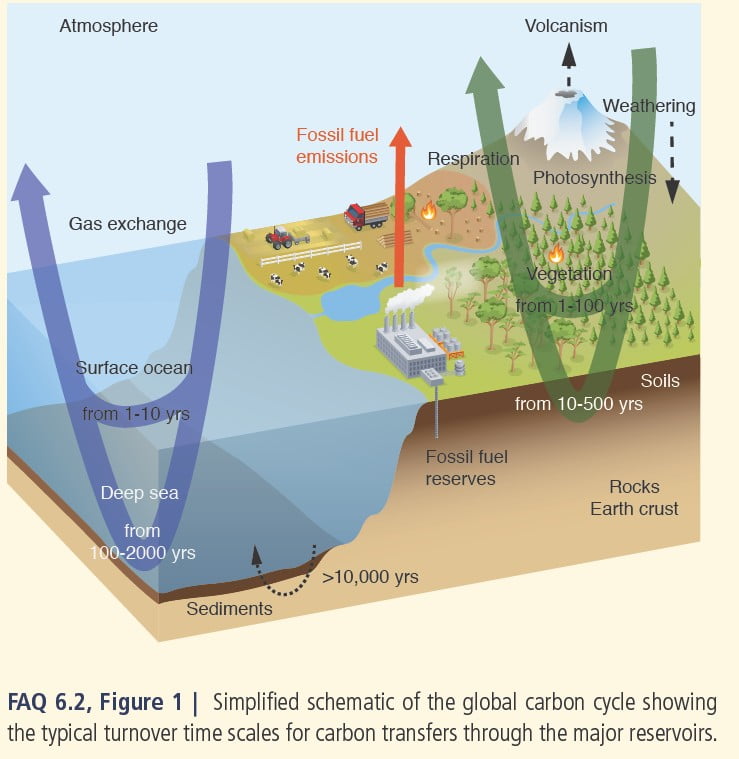
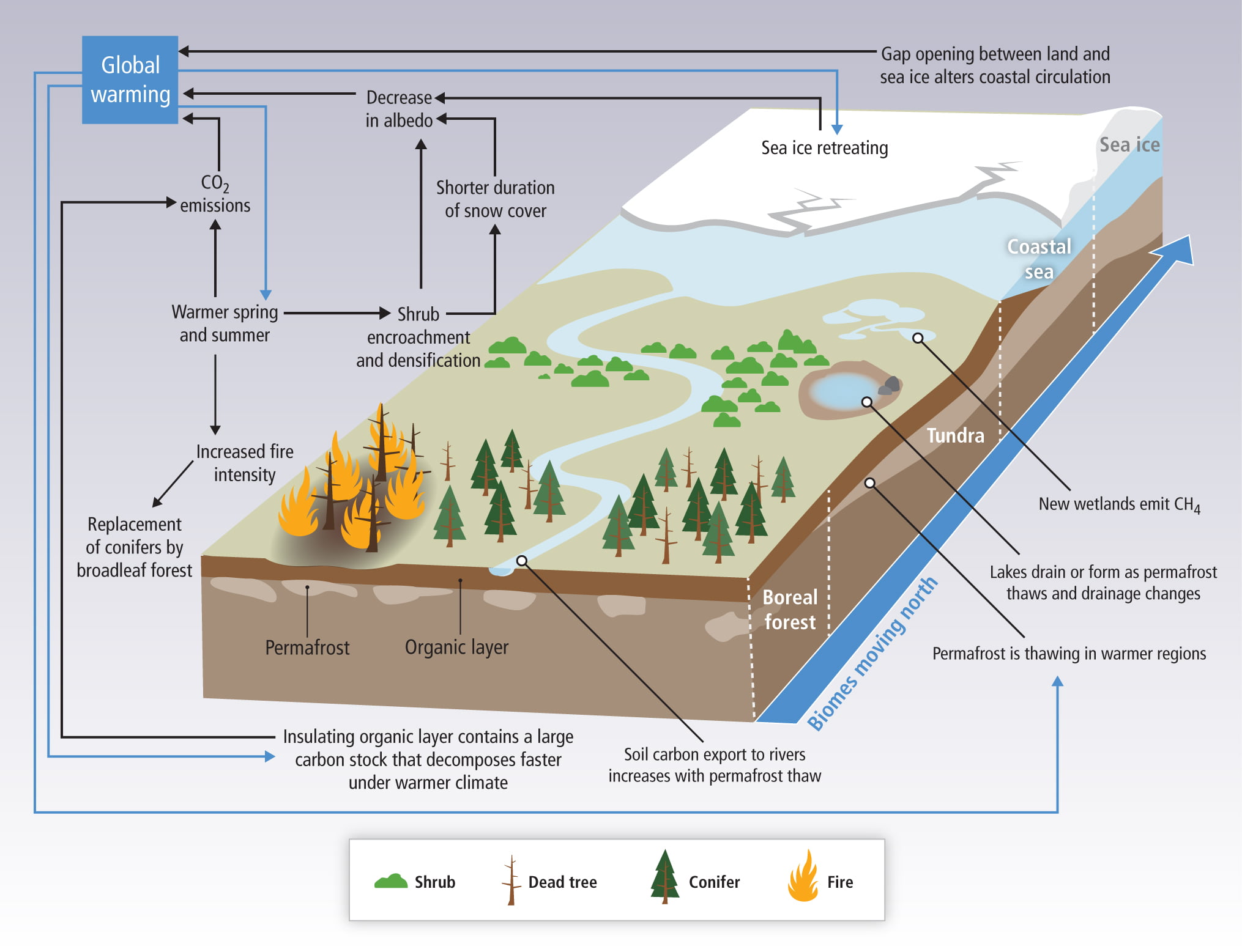
At the moment, vegetation in the Arctic is responsible for about 10% of the CO2 uptake by land globally. Permafrost soils on land and in ocean shelves contain large pools of organic carbon. If permafrost melts, microbes decompose the carbon, releasing it as CO2 or, where oxygen is limited (for example if the soil is covered in standing water), as methane. As the climate of the Arctic warms, more permafrost will thaw. However, warmer Arctic summers would also mean an increase in the amount of vegetation and therefore photosynthesis and CO2 uptake in the Arctic. As yet, scientists don’t know which process will dominate over the next few decades. To complicate matters further, the microbes decomposing the carbon also release heat, causing further melting – a positive feedback.
Methane hydrates are another form of frozen carbon, found in deeper soils. Changes to the temperature and pressure of permafrost soils (and ocean waters) could lead to methane, a gas with a much stronger greenhouse warming potential than carbon dioxide, being released. However, most of the methane is virtually certain to remain trapped underground and will not reach the atmosphere.
The release of carbon dioxide and methane from the Arctic will provide a positive feedback to climate change which will be more important over longer timescales – millennia and longer.
As Arctic and sub-Arctic regions warm more than the global average, the increase in temperature could lead to more regular fire damage to vegetation and soils and carbon release. More generally, increased vegetation cover lowers albedo, meaning that more of the sun’s light is absorbed which in turn warms the climate locally (another positive feedback), as well as increasing evapotranspiration and carbon uptake.