The idea that northerly winds (i.e. winds from the north) are cold, and southerly winds (those from the south) are warm (at least in the northern hemisphere) is quite common. Similarly, air that has travelled over the sea picks up moisture, while air travelling over the land is relatively dry. These simple concepts help in the understanding of air masses. However, as may be expected, there are variations on this theme.
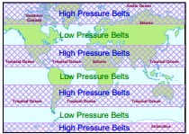
The air in polar and subtropical regions is often within large anticyclones (high pressure areas), during which time it is gradually influenced by the underlying surface – air at the poles is cooled and air in the tropics is warmed. The result is a large body of air with little horizontal variation in temperature and moisture content. Depressions (low pressure areas) develop most frequently in the more temperate latitudes between the pole and the sub-tropics. In doing so, they can cause a large outflow of air from the anticyclones. The warm, sub-tropical air moves into the southern part of the depression, while the cold, polar air, moves into the northern part. These air masses may approach the British Isles, but on their journey, they can be modified by contact with the underlying surface. Air that travels over the sea (maritime air) is moistened, whereas there is little change in moisture content of air that travels over the land (continental air), unless it deposits precipitation (rain or snow). For example, air that has been trapped in an anticyclone over the Sahara in June slowly heats up and dries. After a while, the air moves out of the anticyclone and may head for the British Isles. On its way it may collect moisture over the Mediterranean Sea, but the journey over Spain and France has little effect on its properties. The air then arrives here as a hot, dry air mass.
Air masses affecting the British Isles can be broadly categorised in terms of their source and their path. This leads to four possible types.
Tropical maritime – warm and moist
Tropical continental – warm and dry
Polar maritime – cold and (fairly) moist
Polar continental – cold and dry
To these must be added two further air masses:
Returning polar maritime – which consists of polar air that has moved southwards over the sea and then turns northwards and approaches the British Isles from the south.
Arctic – which consists of air which has travelled southwards from the arctic.
In reality, the type of air mass affecting the British Isles only gives an indication of the type of weather that may occur. The actual weather depends upon the detailed history of the air, the speed of movement and the surface over which it flows.
The boundary between two different types of air mass is referred to as a front. It is common for the British Isles to be affected by a sequence of fronts; usually separating polar maritime and tropical maritime air.
Tropical continental
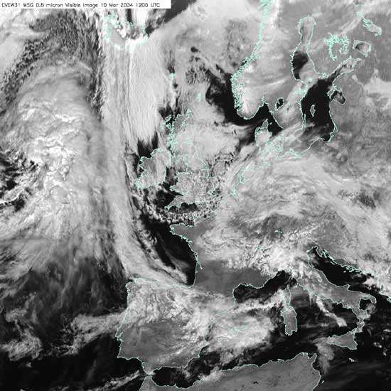
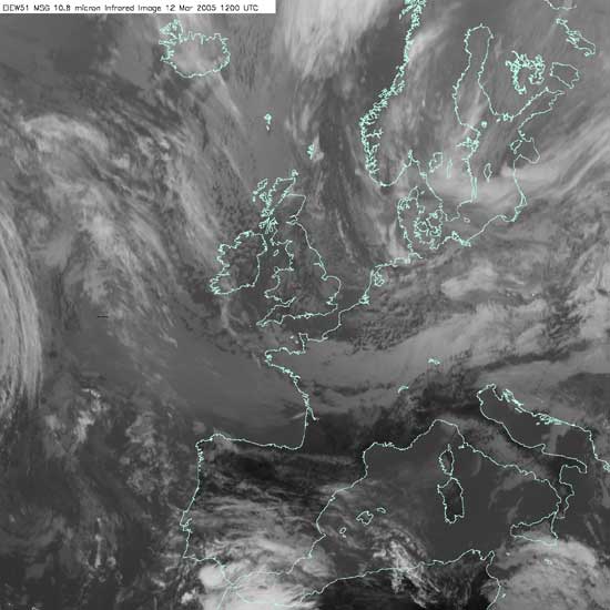
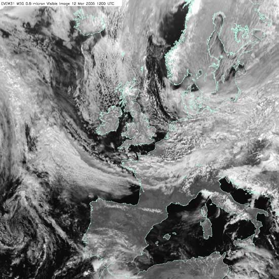
Tropical continental air usually comes with south-easterly or southerly airstreams. It originates in north Africa and often travels over the Mediterranean Sea, Spain and France before reaching the British Isles. In summer, even easterly winds from central Europe or the Ukraine could be included in this category, as the continent becomes so hot at this time of year. The air picks up some moisture over the Mediterranean (and perhaps the Bay of Biscay), but overall the air tends to be quite dry and the skies are typically cloudless.
Strictly speaking, an air mass cooled from below on its northward journey should be stable.
Sometimes, however, moisture may have found its way to medium levels in the atmosphere. Then, if there is a layer of unstable air and a trigger to set off convection, altocumulus castellanus clouds can develop, looking like turrets. These are often the forerunner to tremendous thunderstorms, which can occur by day or night.
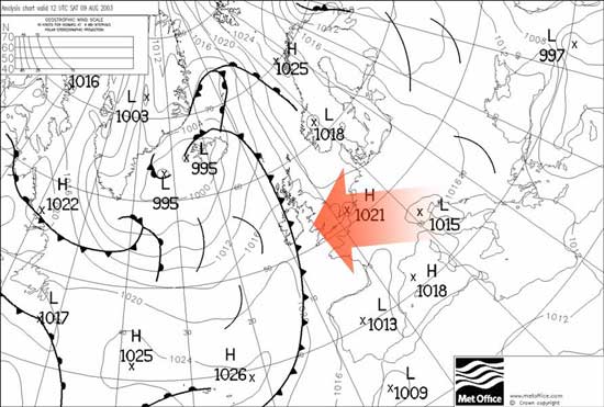
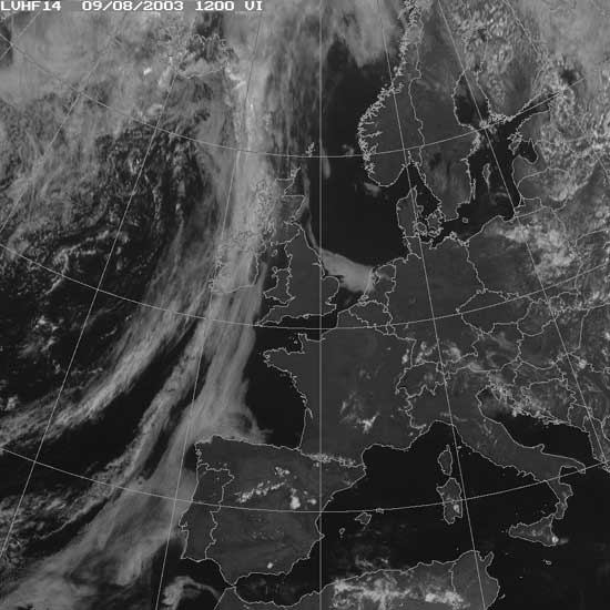
The majority of tropical continental airstreams give a marvellous heatwave (in summer), including the record breaking temperatures of August 2003, although plants and animals tend to be less appreciative of this type of weather.
The lack of moisture usually causes the visibility to be good. However, there may be desert dust, fine soil or pollution particles in the air, which can lead to moderate visibility (often described as ‘heat haze’). Also, the cloudless sky sometimes looks milky because of pollutants.
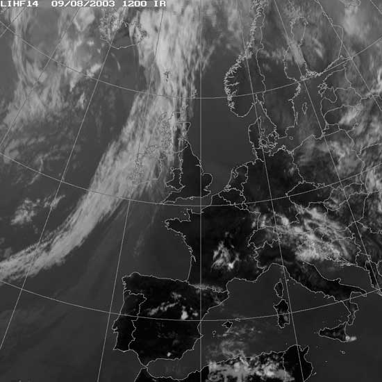
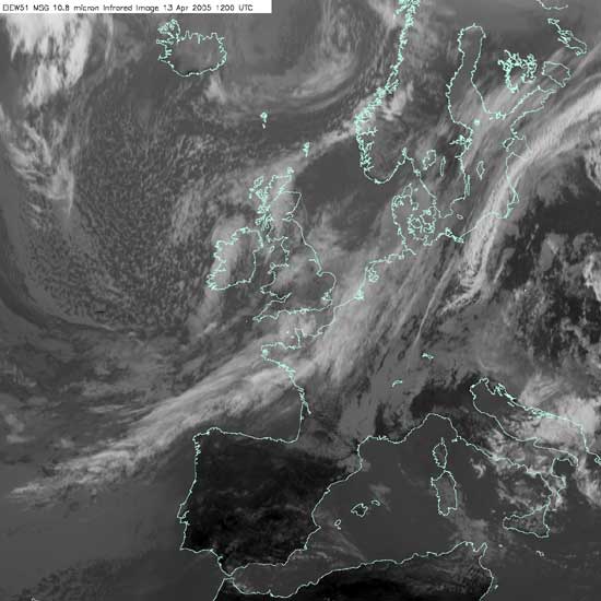
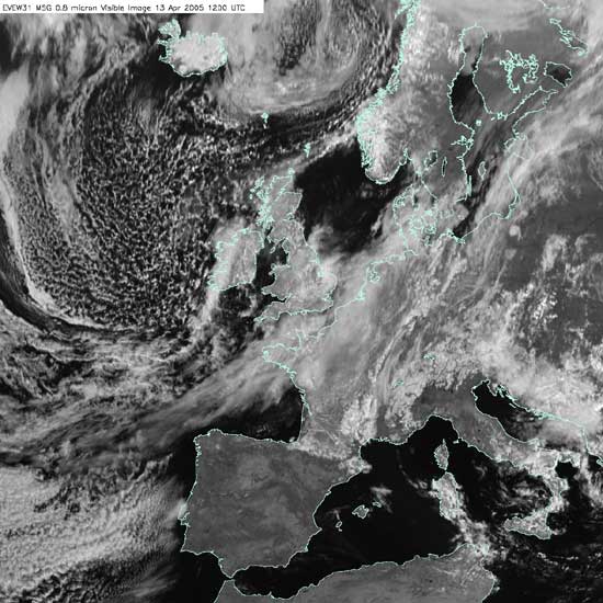
The synoptic chart below shows a typical synoptic situation where the British Isles is being affected by a tropical continental air mass. Both infrared and visible satellite images are also provided for the same time. Click on the images to view a larger version.
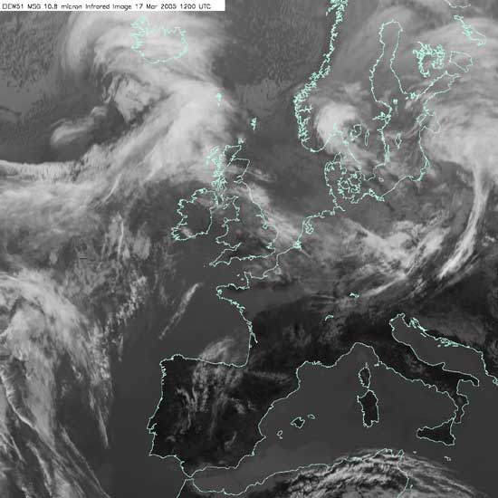
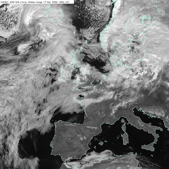
A polar continental air mass originates in Scandinavia or Russia, and reaches the British Isles when north-easterly or easterly winds become established. This tends to occur when there is a high pressure area somewhere to the north of the British Isles, often over Scandinavia itself. Polar continental air masses mainly affect the British Isles during the winter half of the year.
Temperatures in polar continental air masses are below average in winter, except perhaps to the lee of mountains. In summer, however, the temperatures tend to be above average.
The moisture content is low in these air masses, especially when they take the short sea track in the Calais/Dover region. This leads to clouds being generally well broken, and so the weather is fine and sunny.
Air that has crossed the North Sea between Denmark and Scotland is said to have taken a long sea track. It therefore collects more moisture and clouds tend to form during its journey over the sea. Consequently, it is cloudy in eastern districts (with perhaps drizzle or snow flurries), but further inland there tends to be a mixture of cloud and sunshine.
Visibility varies, generally being very good when air comes from Scandinavia, but less good when the air originates in the industrialised regions of central or eastern Europe.
Even in April or May, the North Sea is cold and does little to modify the air mass, apart from adding a little unwelcome moisture. In winter, southern England is particularly chilled by polar continental air masses. Further north, the sea surface makes the air a little less cold and the wind is often less strong.
The synoptic chart below shows a typical synoptic situation where the British Isles is being affected by a polar continental air mass. Both infrared and visible satellite images are also provided for the same time. Click on the images to view a larger version.
Tropical maritime air usually approaches the British Isles from the south-west. Its source region is the subtropical Atlantic Ocean, typically the Azores area, although occasionally it may come almost directly from the Tropics. During its passage across the Atlantic, the air is cooled from below as it passes over a progressively cooler ocean, and so it becomes more stable. While it cools down, little of its moisture is lost. It therefore reaches south-west England or western Ireland almost saturated, giving dull, warm, overcast weather.
On the coasts, sea fog is common in these tropical maritime south-westerlies. However, if the cloud base of the stratus or stratocumulus is several hundred feet, sea-level sites may be saved from the fog, but on rising ground and hills there may be fog and drizzle. Bodmin Moor, Dartmoor, south-west Wales, western Ireland and western Scotland can be shrouded in mild, damp conditions whether it be winter or summer.
Further inland, in the summer half of the year at least, the low stratus may be burnt off by the sun and it could turn out to be quite warm, though still humid. In the lee of hills or mountain ranges, the clouds sometimes break up and there is a lot of sunshine. Favoured locations like north Somerset, North Wales, Northumberland and the Moray Firth can become very warm during summer and bask in spring-like weather on a January day.
Sometimes, an anticyclone may build to the west of the British Isles, keeping the warm, moist air away from western districts and causing it to affect northern Scotland and, sometimes, to move southwards down the east coast. This leads to the formation of haar or fret.
In a tropical maritime air mass, the nights are mild and damp, especially in mid-winter. In December and January, the overcast skies result in little variation in temperature between day and night. However, if there are light winds and clear skies, fog may form inland overnight.
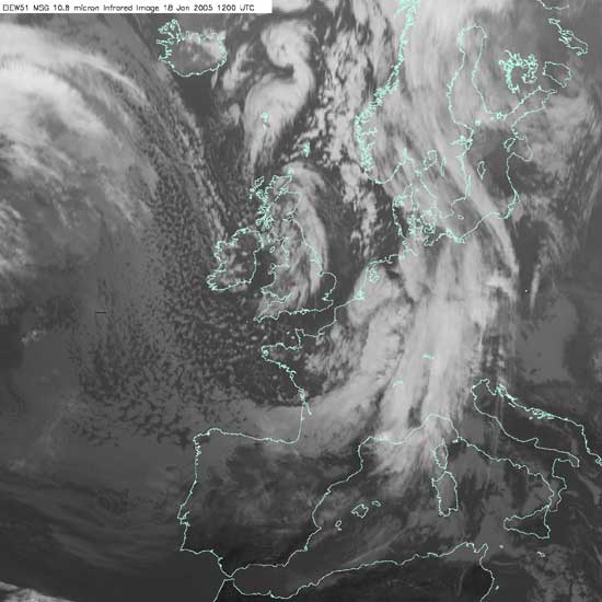
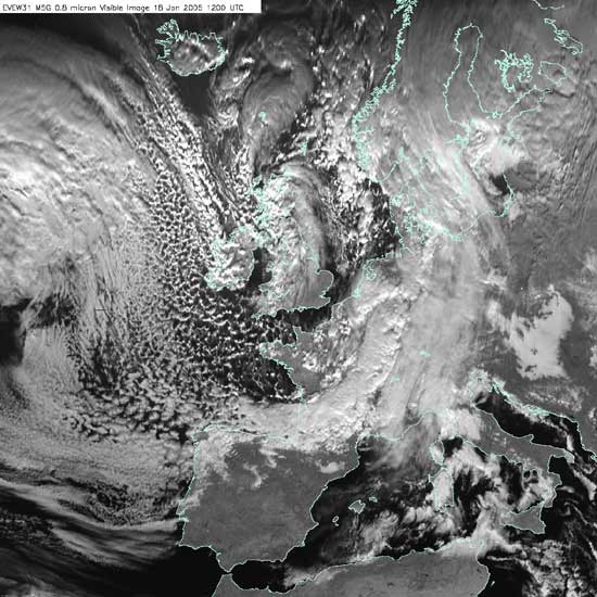
The synoptic chart below shows a typical synoptic situation where the British Isles is being affected by a tropical maritime air mass. Both infra-red and visible satellite images are also provided for the same time. Click on the images to view a larger version.
Polar maritime air is the most common type of air mass affecting the British Isles. The air has its source in the Canadian Arctic or the Greenland area. It reaches the British Isles from the west or north-west after having swung around the western side of a depression. As the cold air travels over the relatively warm sea, it is warmed from below and becomes unstable. Unstable airstreams tend to produce convection, and so cumulus clouds, cumulonimbus clouds and showers are likely in polar maritime air. Other characteristics of the air are that it is cool (especially in summer), fairly moist and associated with good visibility.
In winter, most of the convection is initiated over the Atlantic, and showers hit the coasts, spreading inland if the winds are strong.
The Scottish and Welsh mountains often shelter the eastern side of Britain, although, with a north-westerly wind, some showers sneak through the Cheshire Gap to reach Birmingham and perhaps London.
With a westerly wind, the winter showers can cross Glasgow and central Scotland to reach Edinburgh and Fife; others travel up the Bristol Channel to affect Cardiff and Bristol.
In spring and summer, convection clouds tend to be set off inland by daytime heating. Now, the shelter of the western mountains is less important, and showers or short-lived thunderstorms can occur almost anywhere. At night the clouds disperse.
The synoptic chart below shows a typical synoptic situation where the British Isles is being affected by a polar maritime air mass. Both infrared and visible satellite images are also provided for the same time. Click on the images to view a larger version.
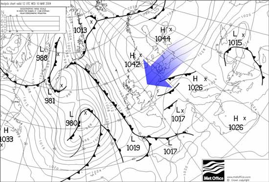
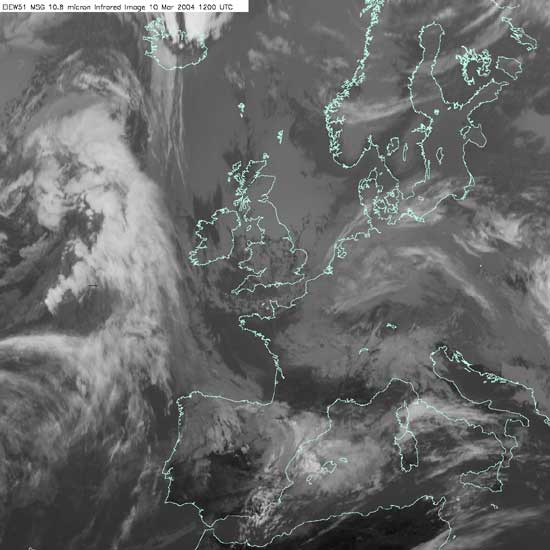
Returning polar maritime air, like polar maritime air, originates in polar regions, but travels southwards before turning north towards the British Isles. The classic returning polar maritime airstream occurs when a large depression is situated somewhere to the north-west of the British Isles. Normally, once the associated weather fronts have passed through, the British Isles are left in a north-westerly polar maritime airstream. However, if the air reaching the British Isles has travelled around the southern edge of the depression and the winds are between south and south-west, the air is designated as returning polar maritime.
The air is originally cold, but as it takes a long sea track southwards across the Atlantic, the lower layers become warmer, more moist and more unstable. However, as it returns northwards, the lower layers are cooled and become more stable. This mixture of a stable layer near the surface and an unstable layer aloft can lead to a wide variety of weather. On exposed coasts and hills, the combination of high moisture content and low-level stability can lead to stratus clouds and hill fog. Sometimes, however, the unstable layer leads to the formation of cumulonimbus clouds and showers (and occasionally thunderstorms). Further inland a mixture of weather can occur – stratus lifts and disperses, allowing heavy showers to form.
South-west England and Wales usually have the first taste of a returning polar maritime airstream; such airstreams are especially common in autumn. Further north and east, with some shelter from the mountains, conditions tend to be better.
East coast areas may well be quite warm, with only broken convection clouds. At night, these areas are usually clear, dry and cool. Moisture contents are quite high, especially near southern coasts, but the clean air usually means good visibility.
Only if the wind becomes very light can inland fog form, where evening showers have moistened the ground.
The synoptic chart below shows a typical synoptic situation where the British Isles is being affected by a returning polar maritime air mass. Both infrared and visible satellite images are also provided for the same time. Click on the images to view a larger version.
Arctic air rarely occurs outside winter and is colder and drier than PM, although it picks up sufficient moisture to produce showers, usually of sleet or snow, on north-facing coasts and hills. As a rule, these showers don’t travel far inland and many places will be fine and sunny, if rather cold. Occasionally, they may become organised into lines of heavy showers and, rarely, into small depressions known as Polar Lows, which can produce quite heavy falls of snow. If accompanied by strong winds, blizzard conditions may develop, usually over the Scottish Highlands.
The synoptic chart below shows a typical synoptic situation where the British Isles is being affected by an arctic air mass. Both infrared and visible satellite images are also provided for the same time. Click on the images to view a larger version.
This information sheet is based on a series of articles written by Dick File that appeared in The Guardian. Web page reproduced with the kind permission of the Met Office
The figure below shows the pressure system over the UK and western Europe on 9 May.
1. What is the name given to the type of front which is running from the southern part of the Baltic Sea inland into Poland?
2. What is the air mass most likely to be associated with this type of front?
3. Where is the source region for this air mass?
4. Describe and explain how the characteristics of this air mass might have changed since it left its source region and passed over the UK and western Europe.
5. What is the name given to the type of front which is running from Scotland east into Scandinavia?
6. What is the air mass most likely to be associated with this type of front?
7. Where is the source region for this air mass?
8. Describe and explain how the characteristics of this air mass might have changed since it left its source region.
9. What further changes might take place as it moves south over Britain?
10. What differences in weather patterns might occur if a tropical continental air mass moved north over the UK at this time of year?
Air masses are parcels of air that bring distinctive weather features to the country. An air mass is a body or ‘mass’ of air in which the horizontal gradients or changes in temperature and humidity are relatively slight. That is to say that the air making up the mass is very uniform in temperature and humidity. An air mass is separated from an adjacent body of air by a transition that may be more sharply defined. This transition zone or boundary is called a front. An air mass may cover several millions of square kilometres and extend vertically throughout the troposphere.
Air masses are parcels of air that bring distinctive weather features to the country. An air mass is a body or ‘mass’ of air in which the horizontal gradients or changes in temperature and humidity are relatively slight. That is to say that the air making up the mass is very uniform in temperature and humidity.
An air mass is separated from an adjacent body of air by a transition that may be more sharply defined. This transition zone or boundary is called a front. An air mass may cover several millions of square kilometres and extend vertically throughout the troposphere.
1.2 Source of an air mass
The temperature of an air mass will depend largely on its point of origin, and its subsequent journey over the land or sea. This might lead to warming or cooling by the prolonged contact with a warm or cool surface. The processes that warm or cool the air mass take place only slowly, for example it may take a week or more for an air mass to warm up by 10 °C right through the troposphere. For this to take place, an air mass must lie virtually in a stagnant state over the influencing region. Hence, those parts of the Earth’s surface where air masses can stagnate and gradually attain the properties of the underlying surface are called source regions.
The main source regions are the high pressure belts in the subtropics, which produce tropical air masses, and around the poles, that are the source of polar air masses.
1.3 Air-mass modification
As we have seen, it is in the source regions that the air mass acquires distinctive properties that are the characteristics of the underlying surface. The air mass may be cool or warm, or dry or moist. The stability of the air within the mass can also be deducted. Tropical air is unstable because it is heated from below, while polar air is stable because it is cooled from below.
As an air mass moves away from its source region towards the British Isles, the air is further modified due to variations in the type or nature of the surface over which it passes. Two processes act independently, or together, to modify an air mass.
An air mass that has a maritime track, i.e. a track predominantly over the sea, will increase its moisture content, particularly in its lower layers. This happens through evaporation of water from the sea surface. An air mass with a long land or continental track will remain dry.
Fig 2: Modification of air mass by land and ocean surfaces
A cold air mass flowing away from its source region over a warmer surface will be warmed from below making the air more unstable in the lowest layers. A warm air mass moving over a cooler surface is cooled from below and becomes stable in the lowest layers.
Fig 3: Modification of air mass due to surface temperature
If we look at the temperature profiles of the previous example, the effects of warming and cooling on the respective air masses are very different.
Fig 4: Modified vertical temperature profiles (—– line) typical of: a) tropical air cooled from below and b) polar air heated from below on its way to the British Isles. Note that where the air is heated from below the effect is spread to a greater depth of the atmosphere.
2.Air mass types
There are four main types of air mass.
Tropical continental (Tc)
Tropical maritime (Tm)
Polar continental (Pc)
Polar maritime (Pm)
And two further sub-divisions.
Arctic maritime (Am)
Returning polar maritime (rPm)
Each of these air-mass types has its own distinctive combination of properties in terms of:
temperature;
moisture content (relative humidity);
change of lapse rate;
stability;
weather;
visibility.
2.1 Tropical continental
Tropical continental air affects the British Isles predominantly during the summer. This air mass affects Britain when pressure is high over northern or eastern Europe with surface winds between east and south drawing hot air from North Africa (see Figure 5). This air is initially unstable but very dry. It acquires some moisture in its passage across the Mediterranean Sea but it is still usually too dry to produce any significant amounts of precipitation. South-westerly winds aloft can sometimes inject sufficient moisture to produce high-based showers or thunderstorms.
Fig 5: Tropical continental air mass
Our highest temperatures usually occur under the influence of tropical continental air (over 30 °C by day and around 15-20 °C at night). Visibility is usually moderate or poor due to the air picking up pollutants during its passage over Europe and from sand particles blown into the air from Saharan dust storms. Occasionally, the Saharan dust is washed out in showers producing coloured rain and leaving cars covered in a thin layer of orange dust.
Tropical continental air may affect the country from March to October, although it is most common in June, July and August. During winter months, tropical continental air is more difficult to identify, but may reach the UK on south or south-easterly winds ahead of slow-moving Atlantic fronts. When high pressure prevails during the winter, strong cooling near the surface makes the air stable, rather than cold and moist. Low cloud and poor visibility may be very persistent under such conditions.
This air mass has a source region over the Eurasian land mass north of 50° N and east of 25° E. It can only be considered a winter phenomenon, as in summer months the land mass becomes very warm, and there are no high-pressure cells develop to ‘push’ the air over the country.
Polar continental air affects the British Isles when pressure is high over Scandinavia with surface winds from an easterly direction (see Figure 6). The characteristics of the air depend on the length of the sea track during its passage from Europe to the British Isles. The air is inherently very cold and dry and it can reach southern Britain after a short sea track over the English Channel, producing weather characterised by clear skies and severe frost. If there is a longer sea track over the North Sea, the air becoming unstable and moisture is added, giving rise to showers of rain or snow. This can be a hazard, especially near the east coast, when the air mass passes over the warmer seas before reaching the colder land surface.
Fig 6: Polar continental air mass
The UK’s lowest temperatures usually occur under this air mass, with temperatures falling below minus 10 °C at night, and sometimes remaining below freezing all day.
Polar continental air only reaches Britain between November and April; at other times of the year, the source region is neither cold nor snow covered and winds from north-eastern Europe bring a more tropical continental form of air.
The source region for this air mass is over the waters of the Atlantic Ocean between the Azores and Bermuda. The air usually reaches the British Isles on south-westerly winds, commonly in the warm sector of a depression or around the periphery of an anticyclone located over central Europe (see Figure 7).
It is warm and moist in its lower layers and during the passage over the cooler waters the air becomes stable and close to saturation. The air mass is modified quickly during its passage across the British Isles and its characteristics vary considerable from place to place depending on exposure to the moist south-westerly flow.
Fig 7: Tropical maritime air mass
In the western parts of the British Isles, the tropical maritime air is stable and saturated in its lowest layers. As a result, the weather is characterised by much low cloud, drizzle and hill fog. During the winter months the air may reach eastern Britain with very similar characteristics providing the ground is cold, but for much of the year insolation is sufficient to warm the air appreciably.
Visibility is more difficult to quantify. When tropical maritime air reaches our western shores it is near to saturation and any uplift produces low cloud and fog which can reduce visibility to near zero. Following a short land track however, and providing the air has dried out appreciably, visibility can become excellent because the air is inherently clear and aerosol free. Following a lengthy land track, haze particles increase in number and are trapped by the stable air reducing visibility to the moderate category.
Polar maritime air flows towards the British Isles on north-westerly winds from the Arctic regions of Greenland and northern Canada. A typical synoptic situation for such an airflow would have a low pressure centred near Iceland (see Figure 8).
This air starts very cold and dry and during its long journey across the comparatively warm waters of the North Atlantic its temperature rises rapidly. The air temperature rises rapidly, allowing it to become unstable to a great depth and causing the moisture content to rise significantly.
Fig 8: Polar maritime air mass
Polar maritime air is perhaps the most familiar air mass. The instability produces showers over the sea, and in the exposed west and north of the British Isles these showers are frequent. In winter months when convection is most vigorous over the sea, hail and thunder are common in these exposed hilly areas. In eastern Britain, where moisture input and surface heating are reduced, showers are less frequent except when troughs of low pressure pass. In the summer months, land temperatures are higher than sea temperatures and the heaviest showers occur over eastern England.
Large variations in shower activity can happen on a diurnal basis as well as on a day-to-day timescale, largely due to subtle changes in stability and moisture content of the air.
Arctic maritime air is a more direct form of Polar maritime. Its source region lies over the Arctic Ocean close to the North Pole.
The synoptic pattern that favours an outbreak of Arctic maritime air is one where high pressure lies to the west of Ireland with low pressure over eastern Europe and southern Scandinavia (see Figure 9). Its characteristics are similar to polar maritime air, but because of the shorter sea track the air is colder and has a lower humidity.
Fig 9: Arctic maritime air mass
Between October and May, the air is cold enough to produce hail showers or snow, and these are most frequent over Scotland and along the coasts exposed to northerly winds. Polar low-pressure systems forming in this air mass can sometimes lead to widespread and heavy snowfall, but otherwise inland areas remain free of cloud in the winter months. In northern Scotland, arctic maritime is usually the coldest air mass, but over the rest of Britain, this air mass is not as cold as polar continental.
Arctic air is uncommon during the summer, but when it does occur it may bring heavy showers or thunderstorms and unseasonably low temperatures.
Returning polar maritime is another variation of polar maritime, but this time, with a much longer sea track which takes the air first southwards over the North Atlantic, then north-eastwards across the British Isles. A typical synoptic pattern associated with this air mass would be a slow moving low pressure in mid-Atlantic with a deep trough extending south (see Figure 10).
During its passage south, the air becomes unstable but on moving north-east it passes over cooler water making it stable in its lower layer whilst remaining unstable aloft.
Fig 10: Returning polar maritime air mass
Tropical continental (Tc)
Polar continental (Pc)
Summer
Winter
Long sea track
Short sea track
Temp
Very warm or hot
Average
Cold
Very cold
Humidity
Relatively dry
Rather moist
Moist in lowest layers
Very dry
Change of lapse rate
Little change
Cooled from below
Heated from below
Little change
Stability
Generally stable
Stable
Unstable
Stable
Weather
Clear, occasional thundery showers
Clear
Rain or snow showers
Clear
Visibility
Moderate or poor
Moderate of poor
Good
Moderate or poor
Tropical maritime (Tm)
Polar Maritime (Pm)
Arctic Maritime (Am)
Returning Polar Maritime (rPm)
Exposed
Sheltered
Temp
Near sea temperature
Warm
Rather cold
Cold (colder than Pm)
Warm (warmer than Pm)
Humidity
Very moist
Moist
Moist
Fairly moist (not as moist as Pm)
Fairly moist (not as moist as Pm)
Change of lapse rate
Cooled from below
Warmed in summer
Heated from below
Heated from below
Heated from below
Stability
Stable
Stable aloft
Unstable
Unstable
Unstable
Weather
Low cloud, drizzle
Broken cloud, dry
Variable cloud, showers
Showers (mainly coastal)
Showers (mainly coastal)
Visibility
Often poor with coastal fog
Moderate
Good
Very good
Very good
Table 1. Typical characteristics of the six major air masses which affect the British Isles.
3. Between the air masses
3.1 Historical introduction
We have looked at the individual types of air masses in some detail, but what is just as, or perhaps, even more important for weather forecasting is what happens in the immediate region where the air masses meet. As we have seen, the air masses have quite different properties so when they meet, perhaps one is cold dry and dry and the other is relatively very warm and moist. These differences produce a reaction in a zone known as a front.
The pioneer in the study of frontal development was Vilhelm Bjerknes, a Norwegian scientist, who analysed their formation around the time of the Great War. The war cut Norway off from outside weather information, so a geophysical institute was founded by Bjerknes in Bergen. He also persuaded the Norwegian government to install a dense network of surface observing stations to provide data for his meteorological studies.
It was known at this time that areas of organised rain were often related to confluence lines in the surface wind field. In 1919, at the age of 22, Vilhelm’s son, Jacob, published an eight-page paper, which introduced the concept of warm, cold and occluded fronts that correctly explained their relationship to extra-tropical depressions.
The term front was introduced as an analogy to the recent war, with air masses, rather than nations, coming together with fronts between air masses compared with the fronts where opposing armies came into contact. By 1926, in collaboration with others at the institute (know collectively as the Bergen School), Bjerknes described the structure and life cycle of frontal depressions.
In recent years, satellites, radar and numerical modelling techniques have provided additional information that has shown that the Norwegian concepts are very simplistic. They do, however, provide a helpful starting point for analysing and forecasting the weather in temperate latitudes.
3.2 Fronts
Fig 11: Vertical cross section through a warm sector of a depression
3.3 Models of mid-latitude depressions
The Bergen School, led by Bjerknes, devised a simple model that shows how depressions, or low pressure systems, develop in mid-latitudes as warm and cold air masses meet. Their model has the following stages.
Origin and infancy – a warm air mass, such as tropical maritime or tropical continental meets a cooler air mass, such as polar maritime or polar continental.
Fig 12: Origin
Maturity – the warm air rises and spirals up in an anticlockwise manner over the sinking cold air. A distinctive warm sector exists between the warm and cold fronts.
Fig 13: Maturity
Occlusion – the warm sector disappears, as the cold front quickly advances. Its faster movement is because the cold front is the leading edge of cold, denser air, pushing up the warmer lighter air. It is harder for the warmer, lighter air at the warm front to cause the cooler, denser air to sink. Hence, the warm front advances at 20 to 30 miles per hour, whilst the cold front can move forward more quickly at 40 to 50 miles per hour.
Fig 14: Occlusion
Death – the frontal system dies as the warm air has completely risen and cooled, and is now underlain by the cold air. The differences in temperature have therefore been equalled out, and the occluded front disappears.
Frontal systems tend to occur in ‘families‘, which migrate in an easterly direction across the Atlantic. Sometimes as many as four or five mature depressions may make their way across the United Kingdom, before a ridge of high pressure builds up to prevent any more from advancing over the country. The origin stage tends to occur over the mid-Atlantic, with the mature stage occurring over the United Kingdom.
The death stage usually occurs over the European mainland and Scandinavia. The depressions follow the zigzag path of the fast jet streams in the upper troposphere. The jet streams may blow at 120 miles per hour in the upper troposphere, but the weather systems below it will usually move more slowly, often at about 40 miles per hour.
Britain’s changeable and damp climate is largely the result of the frequent movement of the rain-bearing fronts across the country. The regularity of their passage, and the standard sequence of changes they produce, allow quite accurate forecasts to be made.
3.4 The passage of a mature depression across the United Kingdom
Fig 15: The passage of a mature depression
The passage of a mature depression across the United Kingdom will produce the following sequence of weather changes.
Ahead of the depression in the cold sector
High cirrus clouds may occur in long feather-like streaks. Some cirrostratus may also occur up to 600 miles ahead of the surface position of the warm front. As the front approaches, temperatures start to rise, and barometric pressure falls steadily.
The warm front passes over
Drizzle and then rain will usually start to fall from altostratus and nimbostratus clouds. The amount of cloud will increase and the cloud base will fall. Continuous rain will persist as pressure carries on falling.
In the warm sector
Pressure stabilises and the amount of cloud falls as the clouds start to thin out. The precipitation also stops, and the weather is generally fine, with a little stratus or stratocumulus. As the cold front approaches, pressures slightly rise and temperatures start to fall slightly.
The cold front passes over
Large, towering cumulonimbus clouds develop as the cold front passes over. This produces heavy downpours of rain and fierce squalls, sometimes with hail and thunder. Pressures rise steadily and air temperatures start to drop as the cold front passes over.
Behind the cold front
There is an end to the heavy rain as the cumulonimbus clouds move away. Barometric pressure continues to rise in a steady fashion. A few showers may occur from some small cumulus clouds, but it is generally fine and cool behind the cold front.
4. Questions
1. Make a simple definition of the following terms. (a) Air mass. (b) Front.
2. Which of the following statements is true? (a) Tropical air is stable because it is heated from below. (b) Tropical air is unstable because it is heated from below. (c) Polar air is stable because it is cooled from below. (d) Polar air is stable because it is heated from below. (e) Polar air is unstable because it is cooled from below.
3. Explain the thermal differences which will occur when: (a) an air mass has a maritime track; (b) a cold air mass moves over a warmer surface.
4. What are the four main types of air mass that affect the UK?
5. Which of the following are the other two subdivisions of air masses which affect the UK? (a) Arctic maritime. (b) Returning polar continental. (c) Returning polar maritime. (d) Arctic continental.
6. Explain how initially dry tropical continental air may acquire enough moisture to produce precipitation.
7. Where is the source region for polar maritime air, and what synoptic situation would allow it to flow over the United Kingdom?
8. Outline the weather features that the UK might experience with returning polar maritime air.
9. Explain why arctic maritime air is likely to lead to good visibility over much of the UK.
10. Which air mass is most associated with thundery showers?
11. Which group of meteorologists first produced a model of frontal development. Was it the: (a) Bristol School, (b) Brighton School, (c) Bergen School, or (d) Berlin School?
12. Why was the term ‘front’ used as an analogy to describe the leading edge of an air mass?
13. Which air mass would move over the UK if pressure was high over Scandinavia and there are surface winds from the east?
14. Which air mass is most likely to produce daytime temperatures, during the summer, in excess of 30 °C?
15. Which air mass is most likely to lead to temperatures at night falling below -10 °C?
16. Outline the features and cloud types associated with the following. (a) Cold front (b) Warm front (c) Occluded front
17. Why does the cold front move faster than the warm front?
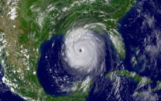
Fig. 1 Satellite Image of Hurricane Katrina, 28 August 2005 at 2045 GMT. Courtesy NOAA/CIMSS/SSEC.
It forms over warm tropical waters where air is rising.
The water must be at least 26°C.
It begins with thunderstorms, then starts to rotate – anti-clockwise in the northern hemisphere and clockwise in the southern hemisphere – with winds of at least 74mph.
It may be five to six miles high and 300 to 400 miles wide (though can be bigger).
It moves forward at speeds of 10-15 mph, but can travel as fast as 40 mph.
These resources explore the climate of five different scale periods of the past 2.6 million years. Within each, some of the basic processes affecting the climate are investigated. Please feel free to adapt the resources to the level and ability of the students you teach.
Module 1 – the last 2.6 million years: Milankovitch Cycles, Supervolcanoes
These resources were jointly produced by Dr Kathryn Adamson (Manchester Metropolitan University), Dr. William Roberts (Bristol University), Dr. Chris Brierley (University College London) and the Royal Meteorological Society.
These resources were Highly Commended by the Geographical Association, who noted that they give teachers structured access to curriculum topics that are otherwise not readily found with up-to-date data from paleo-climate experts.
 Further inland, in the summer half of the year at least, the low stratus may be burnt off by the sun and it could turn out to be quite warm, though still humid. In the lee of hills or mountain ranges, the clouds sometimes break up and there is a lot of sunshine. Favoured locations like north Somerset, North Wales, Northumberland and the Moray Firth can become very warm during summer and bask in spring-like weather on a January day.
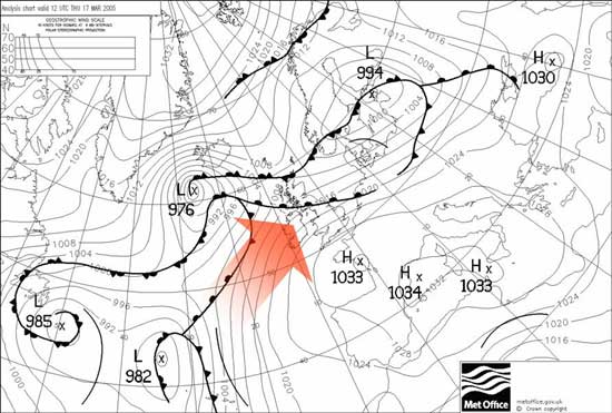
 In winter, most of the convection is initiated over the Atlantic, and showers hit the coasts, spreading inland if the winds are strong.
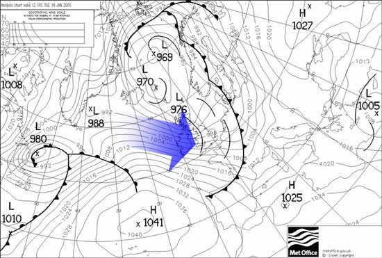
 South-west England and Wales usually have the first taste of a returning polar maritime airstream; such airstreams are especially common in autumn. Further north and east, with some shelter from the mountains, conditions tend to be better.
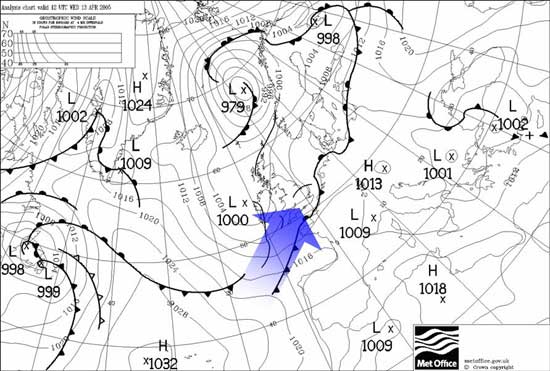


 These resources explore the climate of five different scale periods of the past 2.6 million years. Within each, some of the basic processes affecting the climate are investigated. Please feel free to adapt the resources to the level and ability of the students you teach.