Level: Secondary Geography

secondary-geography

Mitigation Strategies

Post date 9 November 2020

Questions to consider:
Discuss the view that climate change mitigation always requires full international cooperation.
Should all countries have the same goals in their climate policy?

PDF Download

Summary:

Mitigation is a human intervention to limit the amount of climate change for example by reducing the sources or enhancing the sinks of greenhouse gases.
Limiting warming requires substantial technological, economic and institutional challenges.
Mitigation can bring co-benefits to human health and other societal goals
Delaying emissions reduction increases the difficulty and narrows the options for mitigation.
Climate change mitigation requires international cooperation. Effective mitigation will not be achieved if individual countries or groups advance their own interests independently.
Issues of equity, justice, and fairness arise with respect to mitigation and adaptation.

Case Studies

The European Union Emissions Trading Scheme

Developing the Indian Solar Industry

Further Information:

What is the best climate change mitigation policy?

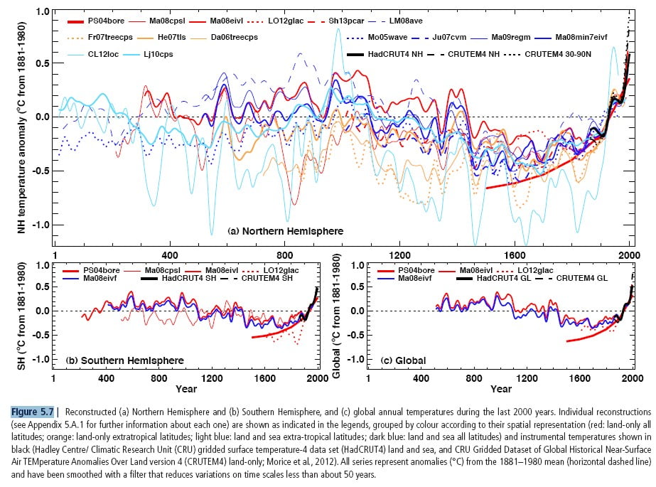
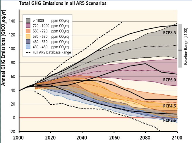WG3 Chapter 6, Figure 7.
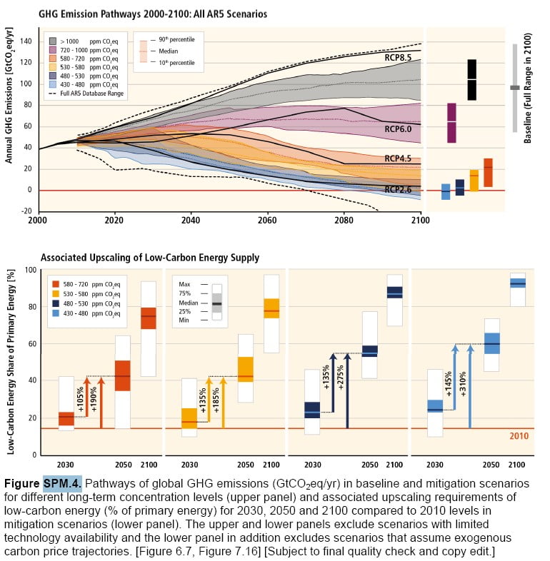
There are many different emissions pathways over the next 85 years which would achieve the same atmospheric greenhouse gas concentration in 2100. For example, to achieve 450 ppm CO₂eq by 2100 (consistent with a likelychance of keeping temperature change below 2°C relative to pre‐industrial levels) a pathway within the pale blue shaded area would have to be followed. Achieving each pathway requires a mix of international and national legislation as well as technological advances.

Scenarios reaching atmospheric concentration levels of about 450 ppm CO₂eq by 2100 (consistent with a likely chance of keeping temperature change below 2°C relative to pre‐industrial levels) include substantial cuts in anthropogenic GHG emissions by mid‐century through large‐scale changes in energy systems and potentially land use. Scenarios reaching these concentrations by 2100 are characterized by lower global GHG emissions in 2050 than in 2010, 40% to 70% lower globally, and emissions levels near zero GtCO₂eq or below in 2100. In scenarios reaching 500 ppm CO₂eq by 2100, 2050 emissions levels are 25% to 55% lower than in 2010 globally. In scenarios reaching 550 ppm CO₂eq, emissions in 2050 are from 5% above 2010 levels to 45% below 2010 levels globally. At the global level, scenarios reaching 450 ppm CO₂eq are also characterized by more rapid improvements of energy efficiency, a tripling to nearly a quadrupling of the share of zero‐ and low‐carbon energy supply from renewables, nuclear energy and fossil energy with carbon dioxide capture and storage (CCS), or bioenergy with CCS by the year 2050. These scenarios describe a wide range of changes in land use, reflecting different assumptions about the scale of bioenergy production, afforestation, and reduced deforestation. All of these emissions, energy, and land‐use changes vary across regions. Scenarios reaching higher concentrations include similar changes, but on a slower timescale. On the other hand, scenarios reaching lower concentrations require these changes on a faster timescale.

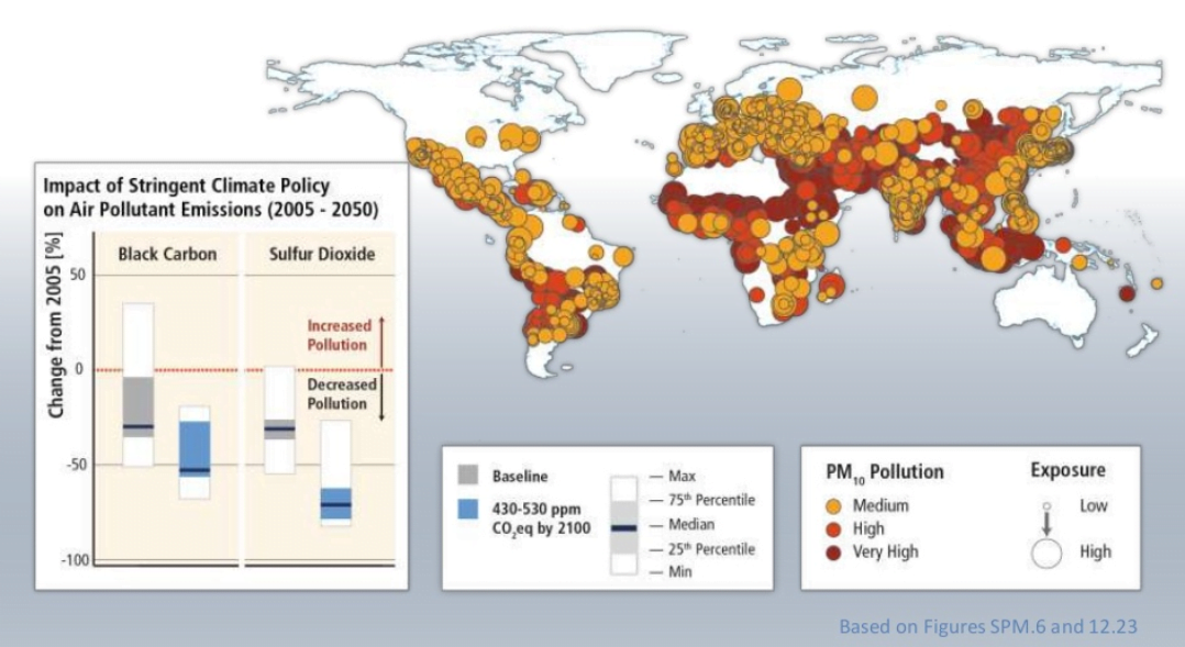
Climate policy – both mitigation and adaptation – can have an impact on other societal goals creating either beneficial (e.g. improving air quality) or adverse side‐effects. These intersections, if well‐managed, can strengthen the case for undertaking climate action. These societal goals, include those related to human health, food security, biodiversity, local environmental quality, energy access, livelihoods, and equitable sustainable development. Conversely, policies directed at other societal goals can influence the achievement of mitigation and adaptation objectives. These influences can be substantial, although sometimes difficult to quantify, especially in welfare terms. A multi‐objective perspective is important in part because it helps to identify areas where support for policies can advance multiple goals.

From IPCC video.
This map shows the exposure of populations to poor air quality, and, in the graph, the side effects of greenhouse gas emission policies on air pollutant emissions (the baseline, grey, scenario is based on legislation currently in place to reduce emissions, the blue scenario involves more stringent legislation).

WG3 Chapter 14, Figure 16.
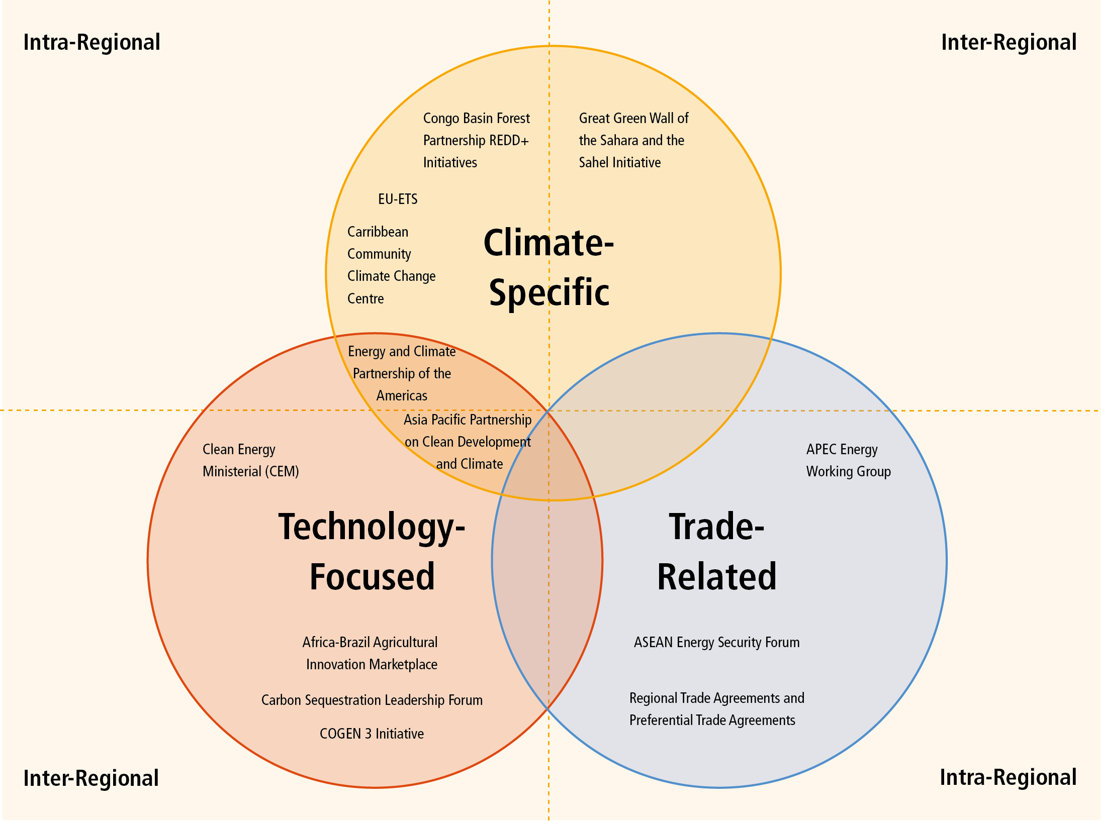
Some regional agreements with mitigation implications – many agreements were not primarily focussed on climate change mitigation, but have achieved emission reductions as an added benefit.

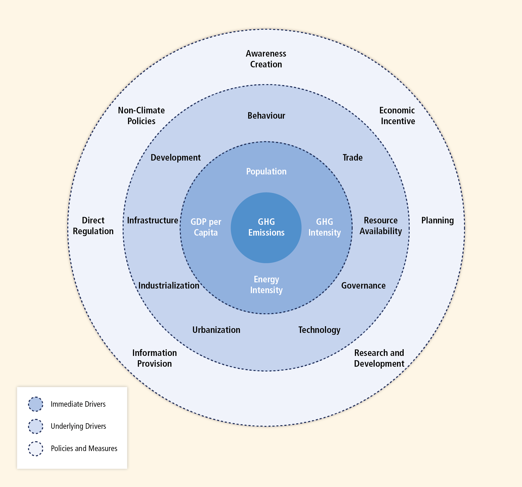WG3 Chapter 5, Figure 1. Interconnections among GHG emissions, immediate drivers, underlying drivers, and policies and measures.
Immediate drivers comprise the factors determining greenhouse gas emissions.
Underlying drivers refer to the processes, mechanisms, and characteristics of society that influence emissions.

Underlying drivers are subject to policies and measures that can be applied to, and act upon them. Changes in these underlying drivers, in turn, induce changes in the immediate drivers and, eventually, in the GHG‐emissions trends. Immediate and underlying drivers may, in return, influence policies and measures.

From IPCC video.In bold, you can see the projected emissions from each sector required to keep total emissions below 450ppm. The baseline scenario (no further mitigation) is shown faintly, where emissions would rise in all sectors except land use.

Could Geoengineering Counteract Climate Change?

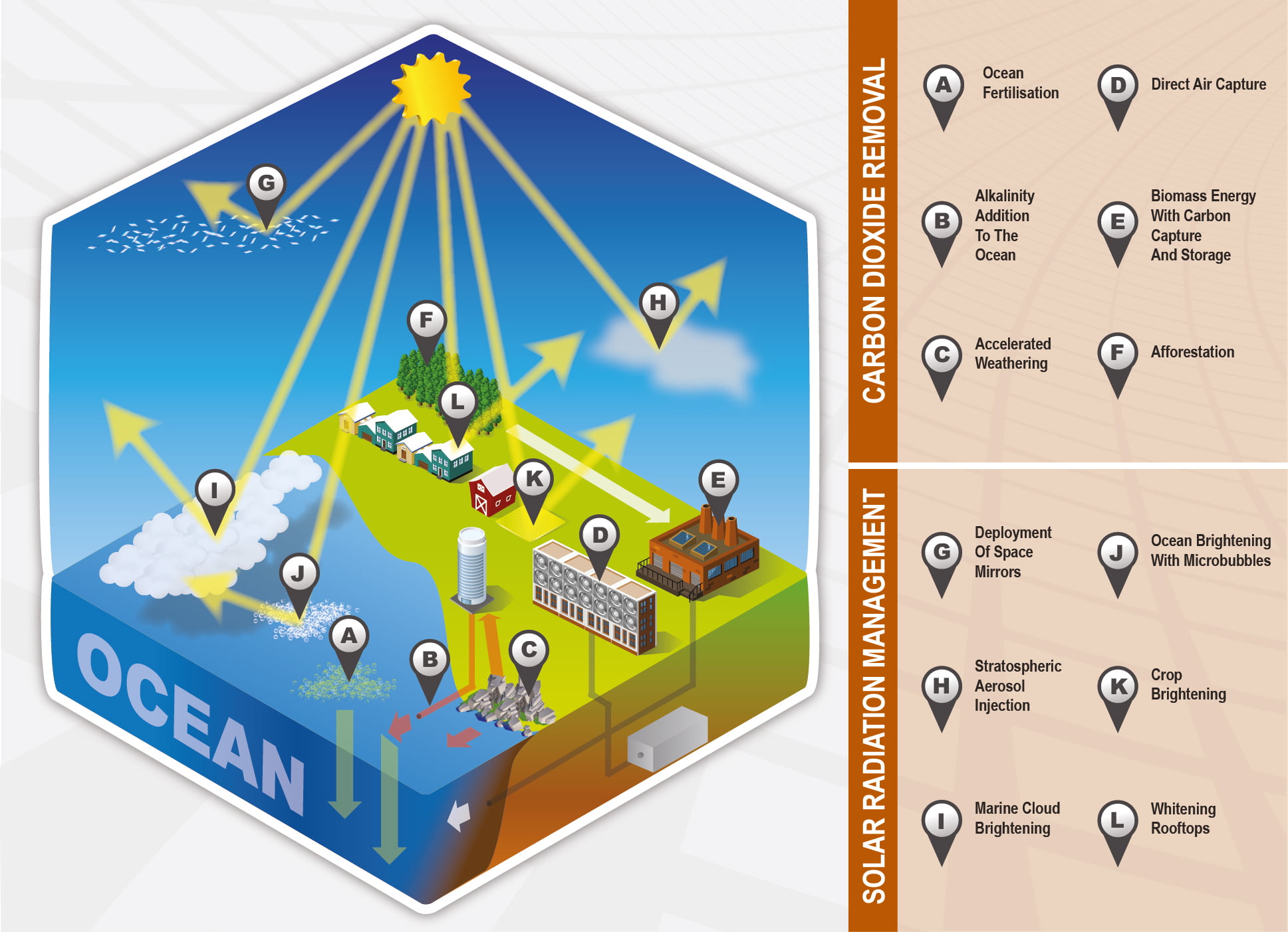
The most direct approach to reducing the effects of anthropogenic climate change is reducing greenhouse gas emissions. However, a number of controversial ‘geoengineering’ approaches have also been proposed as temporary, or additional, interventions. Geoengineering – also called climate engineering – is defined as a broad set of methods and technologies that aim to deliberately alter the climate system in order to alleviate the impacts of climate change.

An overview of some proposed geoengineering methods
Carbon Dioxide Removal methods:
(A) nutrients are added to the ocean (ocean fertilization), which increases oceanic productivity in the surface ocean and transports a fraction of the resulting biogenic carbon downward;
(B) solid minerals which are strong bases add alkalinity to the ocean, which causes more atmospheric CO₂ to dissolve;
(C) the weathering rate of silicate rocks is increased, producing dissolved carbonate minerals which are transported to the ocean;
(D) atmospheric CO₂ is captured chemically, and stored either underground or in the ocean;
(E) biomass is burned at an electric power plant with carbon capture, and the captured CO₂ is stored either underground or in the ocean;
(F) CO₂ is captured through afforestation and reforestation to be stored in land ecosystems.
Solar Radiation Management methods:
(G) reflectors are placed in space to reflect solar radiation;
(H) aerosols are injected in the stratosphere;
(I) marine clouds are seeded in order to be made more reflective;
(J) microbubbles are produced at the ocean surface to make it more reflective;
(K) more reflective crops are grown; and
(L) roofs and other built structures are whitened.
Theory, model simulations and observations suggest that some Solar Radiation Management (SRM) methods which reduce the amount of solar radiation reaching the Earth’s surface could substantially offset a global temperature rise and partially offset some other impacts of climate change. However, regionally, SRM would not precisely offset the temperature and rainfall changes caused by elevated greenhouse gases.
Numerous side effects, risks and shortcomings from SRM have been identified. For example:

SRM might produce a small but significant decrease in global precipitation (with larger differences on regional scales).
Stratospheric aerosol SRM could cause modest polar stratospheric ozone depletion.
As long as GHG concentrations continued to increase, the SRM would also need to increase, exacerbating side effects. In addition, scaling SRM to substantial levels would carry the risk that if the SRM were terminated for any reason, surface temperatures would increase rapidly (within a decade or two) to values consistent with the greenhouse gas forcing, which would stress systems sensitive to the rate of climate change.
SRM would not compensate for ocean acidification from increasing CO₂.
There could also be other as yet unanticipated consequences.

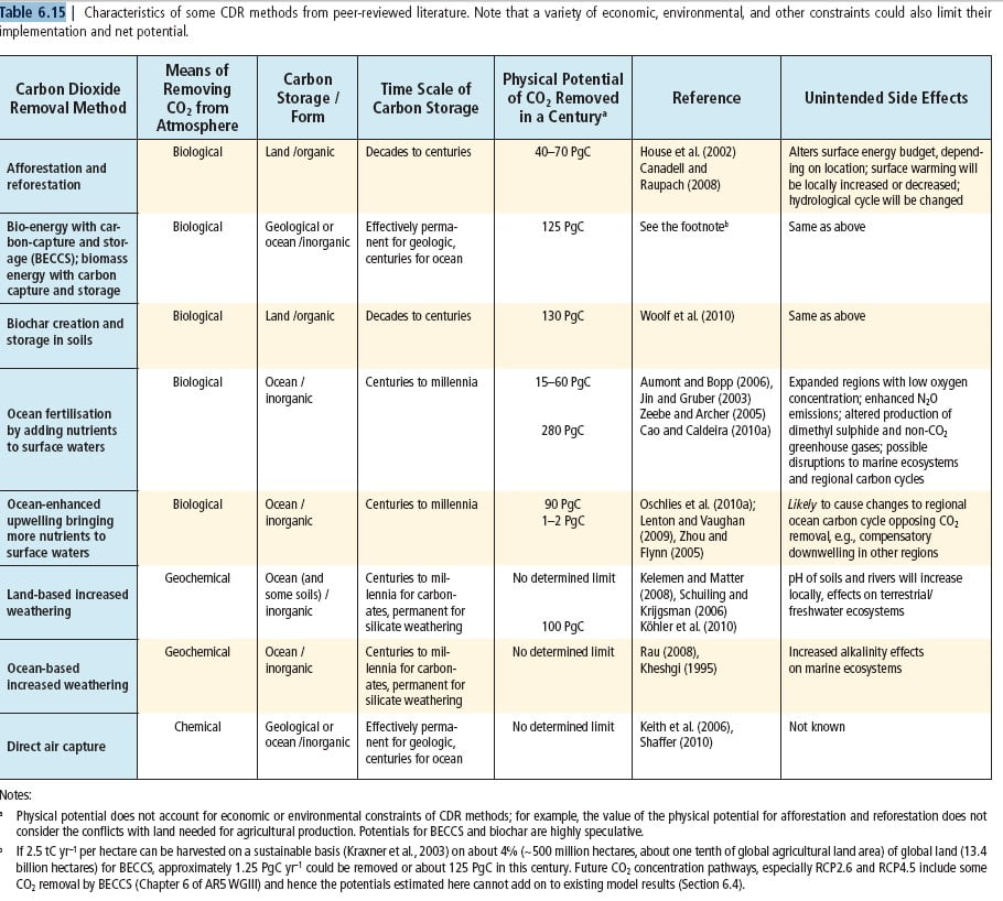
Novel ways to remove CO₂ from the atmosphere on a large scale are termed Carbon Dioxide Removal (CDR) methods. These methods have biogeochemical and technological limitations to their potential. Uncertainties make it difficult to quantify how much CO₂ emissions could be offset by CDR on a human time scale. CDR would probably have to be deployed at large-scale for at least one century to be able to significantly reduce atmospheric CO₂. A major uncertainty is the capacity to store carbon securely with sufficiently low levels of leakage. In addition, it is virtually certain that the removal of CO₂ by CDR will be partially offset by outgassing of CO₂ from the ocean and land ecosystems.
CDR methods can also have associated climatic and environmental side effects:

A large-scale increase in vegetation coverage, for instance through afforestation or energy crops, could alter surface characteristics, such as surface reflectivity. Some modelling studies have shown that afforestation in seasonally snow-covered boreal regions could in fact accelerate global warming, whereas afforestation in the tropics may be more effective at slowing global warming.
Enhanced vegetation productivity may increase emissions of N₂O, which is a more potent greenhouse gas than CO₂.
Ocean-based CDR methods that rely on biological production (i.e. ocean fertilization) would have numerous side effects on ocean ecosystems, ocean acidity and may produce emissions of non- CO₂ greenhouse gases such as methane.

Further Links:
BBC guide to COP21 http://www.bbc.co.uk/news/science-environment-34953626 and, for more information http://www.iea.org/media/news/WEO_INDC_Paper_Final_WEB.PDF
IPCC WG3 video http://www.ipcc.ch/report/ar5/wg3/
IPCC WG3 PowerPoint presentation at http://www.ipcc.ch/report/ar5/wg3/

Link to the COP accord paper http://unfccc.int/resource/docs/2015/cop21/eng/l09.pdf

What is the best climate change mitigation policy?
WG3 FAQ 15.2

A range of policy instruments is available to mitigate climate change including carbon taxes, emissions trading, regulation, information measures, government provision of goods and services, and voluntary agreements. Appropriate criteria for assessing these instruments include: economic efficiency, cost effectiveness, distributional impact, and institutional, political, and administrative feasibility.

Policy design depends on policy practices, institutional capacity and other national circumstances. As a result, there is no single best policy instrument and no single portfolio of instruments that is best across many nations. The notion of ‘best’ depends on which assessment criteria we employ when comparing policy instruments and the relative weights attached to individual criteria. The literature provides more evidence about some types of policies, and how well they score against the various criteria, than others. For example, the distributional impacts of a tax are relatively well known compared to the distributional impacts of regulation. Further research and policy evaluation is required to improve the evidence base in this respect.

Different types of policy have been adopted in varying degrees in actual plans, strategies, and legislation. While economic theory provides a strong basis for assessing economy‐wide economic instruments, much mitigation action is being pursued at the sectoral level. Sectoral policy packages often reflect co‐benefits and wider political considerations. For example, fuel taxes are among a range of sectoral measures that can have a substantial effect on emissions even though they are often implemented for other objectives. Interactions between different policies need to be considered. The absence of policy coordination can affect environmental and economic outcomes. When policies address distinct market failures such as the externalities associated with greenhouse gas emissions or the undersupply of innovation, the use of multiple policy instruments has considerable potential to reduce costs. In contrast, when multiple instruments such a carbon tax and a performance standard are employed to address the same objective, policies can become redundant and undermine overall cost effectiveness.

The European Union Emissions Trading Scheme

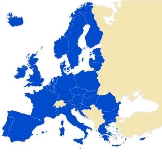The EU Emissions Trading Scheme (ETS), is by far the largest trading scheme worldwide, covering over 12,000 installations belonging to over 4,000 companies and initially over 2 Gt (45%) of annual CO₂ emissions. It puts a cap on the carbon dioxide (CO₂) emitted by business and creates a market and price for carbon allowances, allowing some businesses to pay to emit more than their quota. The cost of buying emissions should drive investment in mitigating technology. It has involved binding and compulsory commitments from its member states together with Norway, Iceland and Liechtenstein. Emissions are estimated to have fallen by 2–5% relative to business‐as‐usual in the first pilot phase from 2005–2007.

In the current phase of the scheme (2013-2020), more industries are being included in the scheme including flights within Europe, and the cap on emissions is being reduced year by year. Compared to 2005, when the EU ETS was first implemented, the proposed cap for 2020 represents a 21% reduction of greenhouse gases. This target has been reached 6 years early. Future reform of the EU ETS will need to clarify the objectives of the scheme, i.e. a quantitative emissions target or a strong carbon price (e.g., to stimulate development of mitigation technologies).

Additional source:

https://en.wikipedia.org/wiki/European_Union_Emission_Trading_Scheme

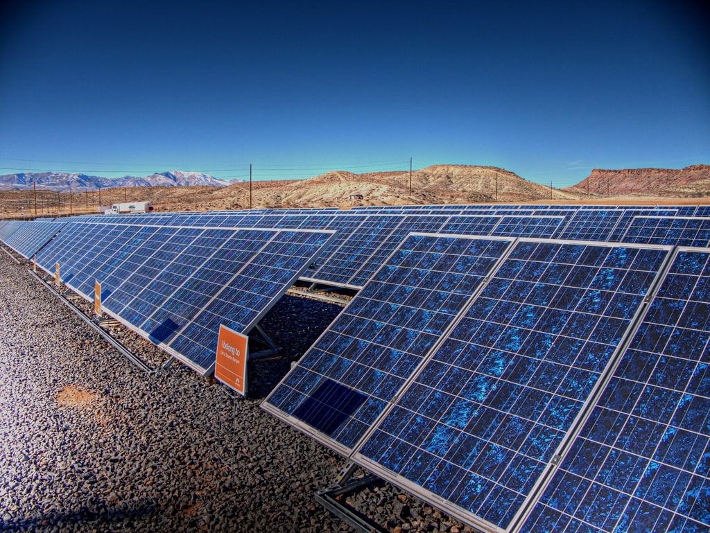
Developing the Indian Solar Industry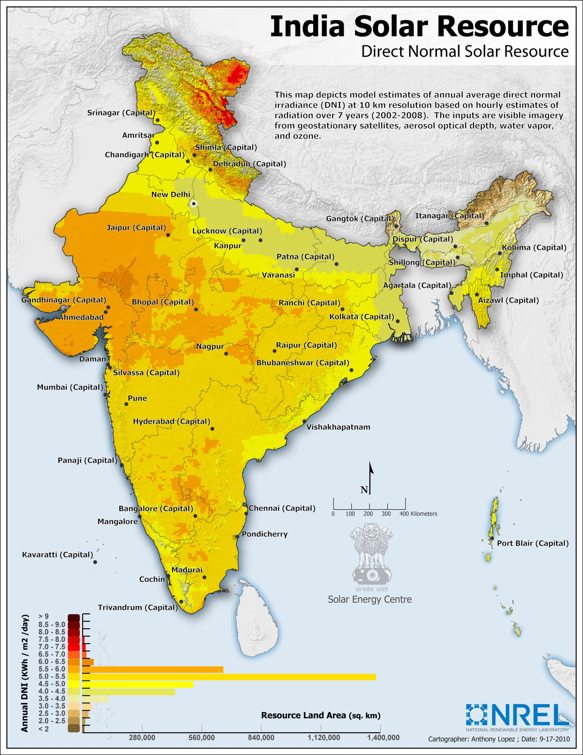

India’s National Action Plan on climate change (NAPCC) identifies eight critical missions to promote climate mitigation and adaptation. One of the core components of this policy, the National Solar Mission, has the specific goal of increasing the usage of solar thermal technologies in urban areas, industry, and commercial establishments. India is a country that has tremendous solar energy potential, receiving nearly 3000 hours of sunshine every year, which is equivalent to 5000 trillion kWh of energy. India can generate over 1,900 billion units of solar power annually, which should be enough to service the entire annual power demand even in 2030. This, coupled with the availability of barren land in the sunniest regions, increases the feasibility of solar energy systems in these regions.

The gap between India’s supply and demand of energy is widening, so developing solar energy helps meet India’s energy needs and also addresses climate mitigation issues. Currently renewable energy supplies only 7.7% of power, mostly through wind. The government has rolled out various policies and subsidy schemes to encourage the growth of the solar industry which also creates a solar manufacturing industry. In January 2015, the Indian government significantly expanded its solar plans, targeting US$100 billion of investment and 100 GW of solar capacity by 2022. It is expected that around 2 GW of solar capacity will be added in 2015. Current limits to growth include the high price of imported silicon.

Additional Source:

Evaluating the Future of Indian Solar Industry http://tejas.iimb.ac.in/articles/75.php

Impact of Climate Change on Water Supplies

Post date 9 November 2020

Questions to consider: What is meant by water security?
How does climate change lead to an increase in water insecurity?
Using a case study, explain one way a country has responded to the threat of water insecurity.

PDF Download

WG2 Chapter 3, Figure 7. The impact of climate change on renewable groundwater resources by the 2050s, for a low emissions scenario. The map also shows the human vulnerability index, which is only defined for areas where the groundwater recharge is projected to decrease by at least 10% relative to 1961-1990.

Summary:

About 80% of the world’s population already suffers serious threats to its water security, as measured by indicators including water availability, demand and pollution.
Climate change is predicted to lead to increased precipitation variability and decreased water storage in snow and ice. In turn, this will lead to increased variability of river flow (including both flooding and drought) which will in turn lead to a less reliable surface water supply.
Each degree of warming is projected to expose an additional 7% of the world population to a 20% or more reduction in their renewable water resources.
By 2050, up to 1 billion people could live in cities with perennial water shortages (less than 100 litres of sustainable surface and groundwater flow per person per day).

Case Studies

Water Saving Irrigation in China

Irrigation in the Upper East Region, Northern Ghana

Return to main menu

Further Information

How will the availability of water resources be affected by climate change?

How should water management be modified in the face of climate change?

Freshwater-related risks of climate change increase significantly with increasing greenhouse gas emissions. Renewable surface water and groundwater resources will be reduced significantly in most dry subtropical regions. Surface and ground water availability has an impact on agriculture (for food and livestock food production), energy production (with a direct impact on hydro-electric power production and crop growth for bioenergy crops as well as on the water cooling for most power plants), domestic water supply and sanitation and freshwater ecosystems.

How will the availability of water resources be affected by climate change?
WG2 FAQ3.2

Climate models project decreases of renewable water resources in some regions and increases in others, albeit with large uncertainty in many places. Broadly, water resources are projected to decrease in many mid-latitude and dry subtropical regions, and to increase at high latitudes and in many humid mid-latitude regions. Even where increases are projected, there can be short-term shortages due to more variable streamflow (because of greater variability of precipitation), and seasonal reductions of water supply due to reduced snow and ice storage. Availability of clean water can also be reduced by negative impacts of climate change on water quality; for instance the quality of lakes used for water supply could be impaired by the presence of algae producing toxins.

In the future, groundwater may be a more reliable water supply than the surface water supply. However, this is only sustainable where, over the long term, withdrawals remain well below recharge, while care must also be taken to avoid excessive reduction of groundwater outflow to rivers. The percentage of the projected global population that will suffer from a decrease of renewable groundwater resources of more than 10% between 1980 and 2080 is projected to be between 24-38%. For each degree of global mean temperature rise, an additional 4% of the global land area is projected to suffer a groundwater resources decrease of more than 30% and an additional 1% to suffer a decrease of more than 70%.

How should water management be modified in the face of climate change?
WG2 FAQ 3.3

Managers of water utilities and water resources have considerable experience in adapting their policies and practices to the weather. But in the face of climate change, long-term planning (over several decades) is needed for a future that is highly uncertain. A flexible portfolio of solutions that produces benefits regardless of the impacts of climate change (“low-regret” solutions) and that can be implemented adaptively, step by step, is valuable because it allows policies to evolve progressively, thus building on – rather than losing the value of – previous investments. Adaptive measures that may prove particularly effective include rainwater harvesting, conservation tillage, maintaining vegetation cover, planting trees in steeply-sloping fields, mini-terracing for soil and moisture conservation, improved pasture management, water re-use, desalination, and more efficient soil and irrigation-water management. Restoring and protecting freshwater habitats, and managing natural floodplains, are additional adaptive measures that are not usually part of conventional management practice.

Water Saving Irrigation in China

Water-saving irrigation (low pressure pipes, spray irrigation and micro or drip irrigation) has enhanced climate change adaptation capacity, improved ecosystem services, and promoted regional sustainable development in China.

Per capita, freshwater availability in China is among the lowest in the world and increasingly in short supply. China’s agriculture currently accounts for 65% of total annual water consumption. With climate change, population growth and a growth in non-agricultural water consumption, China’s agriculture could be faced with a severe shortage of water resources.

Water-saving irrigation, in particular micro-irrigation which drips water directly onto the roots of plants, is one effective measure to deal with water scarcity and food security issues. Through water-saving irrigation practices, the water saved from 2007-2009 was equivalent to 5.6%-11.8% of the national total water consumption.

In addition, about 21.83-47.48 Mt CO₂ emissions were saved (compared to an annual total emission of 6786 Mt CO₂ in 2007). Therefore, the positive benefits of water saving irrigation have included mitigating climate change and promoting sustainable development.

	2007	2008	2009
Water saved (Btu²)	19.37-40.86	19.86-41.55	22.58-57.25
Energy saved (Mt)	2.92-6.39	3.08-6.72	3.57-7.73
CO₂ emission reduction (Mt)	6.66-14.58	7.02-15.31	8.15-17.59

In recent years, a rise in precipitation and temperature has led to the melting of glaciers and expansion of inland high mountain lakes, contributing to alpine grassland degradation in Northern Tibet. Among many grassland protection measures, alpine grassland water saving irrigation measures could be effective in redistributing and making full use of increased precipitation and lake water in the dry period. A three-year demonstration of alpine grassland water saving irrigation measures showed that alpine grassland primary productivity nearly doubled while the number of plant species increased from 91 to 129, helping to protect and restore the alpine grassland ecosystem and ecosystem services and to promote regional, socioeconomically sustainable development.

Additional Source:

Image credit: https://de.wikipedia.org/wiki/Upper_East_Region#/media/File:Ghana-karte-politisch-upper-east.png

Cost-effectiveness analysis of water-saving irrigation technologies based on climate change response: A case study of China, X. Zou, Y. Li, R Cremades, Q. Gao, Y. Wan and X. Qin, 2013, Agricultural Water Management, 129, 9-20.

Irrigation in the Upper East Region, Northern Ghana

The Upper East Region of northern Ghana has, since colonial times (1904-1957), been the poorest part of the country. The area suffers from difficult semi-arid climatic conditions, relatively high population density and patterns of underdevelopment, which are the result of discriminatory colonial and post-colonial policies. Climate change (a decrease in precipitation, increase in temperature and evapotranspiration and a shift in the rainy season) and land degradation have considerably altered the conditions for rain-fed agriculture in Northern Ghana. Furthermore, population pressure has led to continuous farming of the available agricultural lands causing land degradation. Crop failure and decreasing yields that result from these environmental changes have caused further impoverishment. In the past, youth often opted for migration to Ghana’s wealthier south, in order to supplement meagre agricultural livelihoods.

Since the mid-1990s there has been a farmer led initiative to develop shallow groundwater irrigation (SGI) for vegetable gardening of tomatoes, onions and peppers. This development has helped to ameliorate poverty and to reverse rural-urban migration.

However, while the irrigators were initially able to profit from the development of good road access to northern Ghana and an increasing demand for vegetables in Ghana’s south, many now frequently meet with market failure. The sale of fresh tomatoes is met with stiff competition from small-scale farmers from neighbouring Burkina Faso and Ghana’s market is flooded with cheap tomato paste from countries where the production of tomatoes is highly subsidised. Global and regional competition has started to render SGI, developed as a means to locally adapt to environmental change, increasingly risky. As markets become as unreliable as the rains, Ghanaian farmers now face the uphill task of dealing simultaneously with global climate change and globalisation.

Additional Source:

Laube, Wolfram; Awo, Martha; Schraven, Benjamin (2008) : Erratic rains and erratic markets: Environmental change, economic globalisation and the expansion of shallow groundwater irrigation in West Africa, ZEF Working Paper Series, No. 30, http://nbnresolving.de/urn:nbn:de:0202-20080911309
There is a video about managing water resources at https://www.youtube.com/watch?v=R9BB0XdRxEA

Ecosystem Feedbacks from Carbon and Water Cycle Changes

Post date 8 November 2020

carbon, water and nutrient cycle diagram

Questions to consider:
State three factors which would cause a change to the Amazonian Forest Ecosystem.
Explain the impact of the change to the Amazonian Forest Ecosystem
When looking at the effect of climate change on ecosystems, why does the level of carbon dioxide in the atmosphere need to be considered as well as temperature change.

PDF Download

Summary:

Climate change can affect terrestrial and marine ecosystems which in turn has impacts on both the water and carbon cycles and then feeds back to the climate.
Direct human influence on vegetation can also lead to impacts on the climate, through the energy, water and carbon cycles.
Both changes in carbon dioxide and changes in climate have impacts on vegetation.
The interactive effects of elevated CO₂ and other global changes (such as climate change, nitrogen deposition and biodiversity loss) on ecosystem function are extremely complex.
Extreme weather events can have long lasting impacts on vegetation and the carbon and water cycles.

Case Studies

Vegetation changes in the Amazon basin

Return to main menu

Further Information

How do land-use and land-cover changes cause changes in climate?

What are the non-greenhouse gas effects of rising carbon dioxide on ecosystems?

The Carbon Dioxide fertilisation effect

A Possible Amazon Basin Tipping Point

In general, climate exerts a dominant control over the distribution of terrestrial vegetation and surface properties that in turn affects the local climate by changing the local atmospheric water, Carbon and energy budgets. It has been hypothesized that these vegetation–climate feedbacks can explain shifts of vegetation through time: Firstly, increased transpiration may result in more precipitation, which in turn increases plant productivity, which amplifies transpiration further. Secondly, increased productivity leads to more canopy cover, which is darker (lower albedo) than snow and bare soil. This results in higher temperatures on the above ground parts of individual plants, thus also amplifying plant productivity.

The combined effects of a warming climate, higher levels of CO₂, land-use change and increased Nitrogen availability may be responsible for primary productivity increases in many parts of the world. Enhanced productivity can lead to shifts in albedo and transpiration, which feed back to the water cycle through heat fluxes and precipitation.

Rising atmospheric CO₂ concentrations affect ecosystems directly including through biological and chemical processes such as the carbon dioxide fertilisation effect. Plants can respond to elevated CO₂ by opening their stomata less to take in the same amount of CO₂ or by structurally adapting their stomatal density and size, both potentially reducing transpiration which increases the water efficiency of the plants but reduces the flow of water vapour, and the energy that goes with it, to the atmosphere. Paleo records over the Late Quaternary (past million years) show that changes in the atmospheric CO₂ content between 180 and 280 ppmv had ecosystem-scale effects worldwide.

The direct effect of CO₂ on plant physiology, independent of its role as a greenhouse gas, means that assessing climate change impacts on ecosystems and hydrology solely in terms of global mean temperature rise is an oversimplification. A 2°C rise in global mean temperature, for example, may have a different net impact on ecosystems depending on the change in CO₂ concentration accompanying the rise: If a small change in CO₂ causes a 2°C rise, or, if other greenhouse gases are mainly responsible for the rise, the vegetation response will be different to a 2°C rise triggered by a large increase in CO₂.

Vegetation cover can be affected by climate change, with forest cover potentially decreasing (e.g. in the tropics) or increasing (e.g. in high latitudes). In particular, the Amazon forest has been the subject of several studies, generally agreeing that future climate change would increase the risk of tropical forest being replaced by seasonal forest or even savannah. The increase in atmospheric CO₂ reduces the risk, through an increase in the water efficiency of plants.

Direct human changes to the land cover can also have impacts on the carbon and water cycles, as well as on the Earth’s energy balance, through changes in surface albedo, transpiration and evaporation.

The coupling processes between terrestrial Carbon, Nitrogen and hydrological processes are extremely complex and far from well understood.

The effect of climate extremes on vegetation and the carbon and water cycles
Extreme events such as heatwaves, droughts and storms can cause vegetation death, fires and subsequent insect infestations which actually lead to a net output of carbon from ecosystems. For example, forests are characterized by the large biomass carbon stocks, which are vulnerable to wind damage, storms, ice storms, frost, drought, fire and pathogen or pest outbreaks. Trees take a long time to regrow, so the recovery times for forest biomass lost through extreme events are particularly long. Therefore, the effects of climate extremes on the carbon balance in forests are both immediate and lagged, and potentially long-lasting. Climate extremes may also trigger processes that decrease the turnover rate of some carbon pools and lead to additional long-term sequestration in these pools. A well-known example is charcoal created in fires, which generally persists longer in soils than leaf litter.

During the European 2003 heatwave, it was the lack of precipitation (and soil moisture) rather than the high temperatures which was the main factor limiting vegetation growth in the temperate and Mediterranean forest ecosystems.

Further Links:

There is a nice, short summary article at http://www.carbonbrief.org/blog/2011/03/new-scientific-papers-on-plants-and-carbon-dioxide/
http://www.nature.com/nature/journal/v500/n7462/fig_tab/nature12350_F2.html An overview of how carbon flows may be triggered, or greatly altered, by extreme events including extreme precipitation.

Figure 1 from http://www.mdpi.com/1424-8220/9/11/8624/htm shows a schematic view of the components of the climate system, their processes and interactions.

Ocean related feedback exists between climate variability, the water cycle and the carbon cycle. http://nasa-information.blogspot.co.uk/2010/11/ocean-earth-system.html
http://www.nasa.gov/images/content/703470main_InfoGraphic.jpg An infographic showing the limits to vegetation growth from soil nutrient availability.

A figure showing the ecosystem processes and feedbacks triggered by extreme climate events. http://www.nature.com/nature/journal/v500/n7462/fig_tab/nature12350_F1.html

How do land-use and land-cover changes cause changes in climate?
WG2 FAQ 4.1

Land use change affects the local as well as the global climate. Different forms of land cover and land use can cause warming or cooling and changes in rainfall, depending on where they occur in the world, what the preceding land cover was, and how the land is now managed. Vegetation cover, species composition and land management practices (such as harvesting, burning, fertilizing, grazing or cultivation) influence the emission or absorption of greenhouse gases. The brightness of the land cover affects the fraction of solar radiation that is reflected back into the sky, instead of being absorbed, thus warming the air immediately above the surface. Vegetation and land use patterns also influence water use and evapotranspiration, which alter local climate conditions. Effective land-use strategies can also help to mitigate climate change.

What are the non-greenhouse gas effects of rising carbon dioxide on ecosystems?
WG2 FAQ 4.2

Carbon dioxide (CO₂) is an essential building block of the process of photosynthesis. Simply put, plants use sunlight and water to convert CO₂ into energy. Higher CO₂ concentrations enhance photosynthesis and growth (up to a point), and reduce the water used by the plant. This means that water remains longer in the soil or recharges rivers and aquifers. These effects are mostly beneficial; however, high CO₂ also has negative effects, in addition to causing global warming. High CO₂ levels cause the nitrogen content of forest vegetation to decline and can increase their chemical defences, reducing their quality as a source of food for plant-eating animals. Furthermore, rising CO₂ causes ocean waters to become acidic, and can stimulate more intense algal blooms in lakes and reservoirs.

The Carbon Dioxide fertilisation effect
WG1 Box 6.3

Elevated atmospheric CO₂ concentrations lead to higher leaf photosynthesis and reduced canopy transpiration, which in turn lead to increased plant water use efficiency and reduced fluxes of latent heat from the surface to the atmosphere. The increase in leaf photosynthesis with rising CO₂, the so-called CO₂ fertilisation effect, plays a dominant role in terrestrial biogeochemical models to explain the global land carbon sink, yet it is one of most unconstrained process in those models.

Field experiments provide a direct evidence of increased photosynthesis rates and water use efficiency (plant carbon gains per unit of water loss from transpiration) in plants growing under elevated CO₂. These physiological changes translate into a broad range of higher plant carbon accumulation in more than two-thirds of the experiments and with increased net primary productivity (NPP) of about 20 to 25% at double CO₂ from pre-industrial concentrations. Since the last IPCC report, new evidence is available from long-term Free-air CO₂ Enrichment (FACE) experiments in temperate ecosystems showing the capacity of ecosystems exposed to elevated CO₂ to sustain higher rates of carbon accumulation over multiple years. However, FACE experiments also show the diminishing or lack of CO₂ fertilisation effect in some ecosystems and for some plant species. This lack of response occurs despite increased water use efficiency, also confirmed with tree ring evidence

Nutrient limitation is hypothesized as primary cause for reduced or lack of CO₂ fertilisation effect observed on NPP in some experiments. Nitrogen and phosphorus are very likely to play the most important role in this limitation of the CO₂ fertilisation effect on NPP, with nitrogen limitation prevalent in temperate and boreal ecosystems, and phosphorus limitation in the tropics. Micronutrients interact in diverse ways with other nutrients in constraining NPP such as molybdenum and phosphorus in the tropics. Thus, with high confidence, the CO₂ fertilisation effect will lead to enhanced NPP, but significant uncertainties remain on the magnitude of this effect, given the lack of experiments outside of temperate climates.

A Possible Amazon Basin Tipping Point
WG2 Box 4.3

Since the last assessment report of the IPCC (AR4), our understanding of the potential of a large-scale, climate-driven, self-reinforcing transition of Amazon forests to a dry stable state (known as the Amazon “forest dieback”) has improved. Modelling studies indicate that the likelihood of a climate-driven forest dieback by 2100 is lower than previously thought, although lower rainfall and more severe drought is expected in the eastern Amazon. There is now medium confidence that climate change alone (that is, through changes in the climate envelope, without invoking fire and land use) will not drive large-scale forest loss by 2100 although shifts to drier forest types are predicted in the eastern Amazon.

Meteorological fire danger is projected to increase. Field studies and regional observations have provided new evidence of critical ecological thresholds and positive feedbacks between climate change and land-use activities that could drive a fire mediated, self-reinforcing dieback during the next few decades. There is now medium confidence that severe drought episodes, land use, and fire interact synergistically to drive the transition of mature Amazon forests to low-biomass, low-statured fire-adapted woody vegetation. Most primary forests of the Amazon Basin have damp fine fuel layers and low susceptibility to fire, even during annual dry seasons. Forest susceptibility to fire increases through canopy thinning and greater sunlight penetration caused by tree mortality associated with selective logging, previous forest fire, severe drought, or drought-induced tree mortality. The impact of fire on tree mortality is also weather-dependent. Under very dry, hot conditions, fire-related tree mortality can increase. Under some circumstances, tree damage is sufficient to allow light-demanding, flammable grasses to establish in the forest understorey, increasing forest susceptibility to further burning. There is high confidence that logging, severe drought, and previous fire increase Amazon forest susceptibility to burning. Landscape level processes further increase the likelihood of forest fire. Fire ignition sources are more common in agricultural and grazing lands than in forested landscapes, and forest conversion to grazing and crop lands can inhibit regional rainfall through changes in albedo and evapotranspiration or through smoke that can inhibit rainfall under some circumstances. Apart from these landscape processes, climate change could increase the incidence of severe drought episodes.

If recent patterns of deforestation (through 2005), logging, severe drought, and forest fire continue into the future, more than half of the region’s forests will be cleared, logged, burned or exposed to drought by 2030, even without invoking positive feedbacks with regional climate, releasing 20±10 Pg of carbon to the atmosphere. The likelihood of a tipping point being reached may decline if extreme droughts (such as 1998, 2005, and 2010) become less frequent, if land management fires are suppressed, if forest fires are extinguished on a large scale, if deforestation declines, or if cleared lands are reforested. The 77% decline in deforestation in the Brazilian Amazon with 80% of the region’s forest still standing demonstrates that policy-led avoidance of a fire-mediated tipping point is plausible.

WG2 Chapter 4, Figure 8.
The forests of the Amazon Basin are being altered through severe droughts, land use (deforestation, logging), and increased frequencies of forest fire. Some of these processes are self-reinforcing through positive feedbacks, and create the potential for a large-scale tipping point. For example, forest fire kills trees, increasing the likelihood of subsequent burning. This effect is magnified when tree death allows forests to be invaded by grasses, which are more flammable. Deforestation provides ignition sources to flammable forests, contributing to this dieback. Climate change contributes to this tipping point by increasing drought severity, reducing rainfall and raising air temperatures, particularly in the eastern Amazon Basin.

Vegetation changes in the Amazon basin

WG2 Chapter 4, Figure 8. The forests of the Amazon Basin are already being altered through severe droughts, changes in land use (deforestation, logging), and increased frequencies of forest fire. Some of these processes are self-reinforcing through positive feedbacks, and create the potential for a large-scale tipping point. For example, forest fire kills trees, increasing the likelihood of subsequent burning. This effect is magnified when tree death allows forests to be invaded by flammable grasses. Deforestation provides ignition sources to flammable forests, contributing to this dieback. Climate change contributes to this tipping point by increasing drought severity, reducing rainfall and raising air temperatures, particularly in the eastern Amazon Basin.

There is a high risk that the large magnitudes and high rates of climate change this century will result in abrupt and irreversible regional-scale changes to terrestrial and freshwater ecosystems, especially in the Amazon and Arctic, leading to additional climate change.

There are plausible mechanisms, supported by experimental evidence, observations, and climate model simulations, for the existence of ecosystem tipping points in the rainforests of the Amazon basin. Climate change (temperature and precipitation changes) alone is not projected to lead to abrupt widespread loss of forest cover in the Amazon during this century. However, a projected increase in severe drought episodes, related to stronger El Niño events, together with land-use change and forest fires, would cause much of the Amazon forest to transform to less dense, drought- and fire-adapted ecosystems. This would risk reducing biodiversity in an important ecosystem, and would reduce the amount of carbon absorbed from the atmosphere through photosynthesis. It would also reduce the amount of evaporation, increasing the warming locally. Large reductions in deforestation, as well as wider application of effective wildfire management would lower the risk of abrupt change in the Amazon.

Amazonian forests were estimated to have lost 1.6 PgC and 2.2 PgC following the severe droughts of 2005 and 2010, respectively.

A Possible Amazon Basin Tipping Point

Deforestation, the water cycle and the carbon cycle in the Amazon – learning ideas related to this.

Additional source:

Climate extremes and the carbon cycle, M. Reichstein, M. Bahn, P. Ciais, D. Frank, M. Mahecha, S. Seneviratne,.J. Zscheischler, C. Beer, N. Buchmann, D. Frank, D. Papale, A. Rammig, P. Smith, K. Thonicke, M. van der Velde, S. Vicca, A. Walz & M. Wattenbach, 2013, 500, Nature, 287-295.

Cool Geography

Country-by-Country Emissions of Greenhouse Gases

Post date 8 November 2020

emissions map — Carbon Emissions Map, resizing the territories according to their proportion of global carbon dioxide emissions and colouring them according to their per capita emissions. Reproduced with permission from Dr. Benjamin Hennig http://www.viewsoftheworld.net/ .

Questions to consider: Describe the global distribution of carbon emissions
Explain the reasons for the high proportion of global carbon dioxide emissions for one country shown on the carbon emissions map.

PDF Download

Summary:

The increase in CO₂ emissions from both fossil fuel burning and land use change are the dominant cause of the observed increase in atmospheric CO₂ concentration, which is now over 40% above pre-industrial levels.
Global CO₂ emissions have continued to grow over the last 10 years, but there are large variations in emission trajectories between countries.
The Ocean has absorbed about 30% of the emitted anthropogenic carbon dioxide.
Anthropogenic CO₂ emissions are currently closest to the highest emissions scenario the IPCC considered.

Case Studies

Reducing greenhouse gas emissions in Germany, an Advanced Country (AC)

Reducing greenhouse gas emissions in the USA, an Advanced Country (AC)

Reducing greenhouse gas emissions in China, an Emerging and Developing Country (EDC)

Reducing greenhouse gas emissions in Poland, an Emerging and Developing Country (EDC)

Return to main menu

Further Information

Figure reproduced with permission from the Global Carbon Atlas: globalcarbonatlas.org
Data sources CDIAC: Boden, TA, G Marland, and RJ Andres. 2013. Global, Regional, and National Fossil-Fuel CO2 Emissions. Carbon Dioxide Information Analysis Center (CDIAC), Oak Ridge National Laboratory, US Department of Energy, Oak Ridge, Tenn., USA doi:10.3334/CDIAC/00001_V2013 http://cdiac.ornl.gov/trends/emis/meth_reg.html and UN: United Nations Population Division – World Population Prospects: The 2012 Revision, 2013 http://esa.un.org/unpd/wpp/Excel-Data/population.htm

What Happens to Carbon Dioxide After It Is Emitted into the Atmosphere?

Annual anthropogenic CO₂ emissions and their partitioning among the atmosphere, land and ocean (PgC yr–1) from 1750 to 2011. (Top) Fossil fuel and cement CO₂ emissions by category (Bottom) Fossil fuel and cement CO₂ emissions, CO₂ emissions from net land use change (mainly deforestation), the atmospheric CO₂ growth rate, the ocean CO₂ sink and the residual land sink which represents the sink of anthropogenic CO₂ in natural land ecosystems. The emissions and their partitioning only include the fluxes that have changed since 1750, and not the natural CO₂ fluxes (e.g., atmospheric CO₂ uptake from weathering, outgassing of CO₂ from lakes and rivers, and outgassing of CO₂ by the ocean from carbon delivered by rivers) between the atmosphere, land and ocean reservoirs that existed before that time and still exist today. WG1 Chapter 6, Figure 8.

Anthropogenic CO₂ emissions to the atmosphere were 555 ± 85 PgC between 1750 and 2011. Of this, fossil fuel combustion and cement production contributed 375 ± 30 PgC and land use change (including deforestation, afforestation (planting new forest) and reforestation) contributed 180 ± 80 PgC. In 2002–2011, average fossil fuel and cement manufacturing emissions were 7.6 to 9.0 PgC/ year, with an average increase of 3.2%/ year compared with 1.0%/ year during the 1990s. In 2011, fossil fuel emissions were in the range of 8.7 to 10.3 PgC.

Emissions due to land use changes between 2002 and 2011 are dominated by tropical deforestation, and are estimated to range between 0.1 to 1.7 PgC/year. This includes emissions from deforestation of around 3 PgC/ year compensated by an uptake of around 2 PgC/year by forest regrowth (mainly on abandoned agricultural land).
The IPCC concluded that the increase in CO₂ emissions from both fossil fuel burning and land use change are the dominant cause of the observed increase in atmospheric CO₂ concentration.

Reducing greenhouse gas emissions in Germany, an Advanced Country (AC)

Between 1990 and 2014, most major German sources of emissions achieved CO₂ reductions. In the energy industry sector, which is responsible for the largest share (around 40%) of Germany’s greenhouse gas emissions, emissions fell by 24% between 1990 and 2014. Even bigger reductions were achieved by households (32.9 %) and industry (33.8 %), helped by the fall of the Berlin wall and the subsequent decline of East German industry and power production and the 2009 economic crisis. The transport sector only reduced its emissions by 0.2 %.
Around half of German electricity is still produced in coal- and gas-fired power plants but Germany is pushing ahead with its transition to renewable energy sources. The production costs of renewable energy have dropped by 70% in the past 5 years, making them a much more competitive energy source. In 2015 the share of renewables in the country’s domestic energy mix increased to 33%,
At the same time, Germany managed to cut down its power consumption in the past year by 3.8%, despite a booming economy (+1.4 %) which generally translates into a higher energy demand, by using LED technology and energy saving measures. CO₂ emissions correspondingly fell by 5%. However, 4% of that figure is linked to mild weather conditions requiring less heating.
In 2011, Germany took 8 nuclear power plants off the grid after the Fukushima disaster.
Germany aims to cut greenhouse gas emissions by 40% by 2020 and up to 95% in 2050. It may struggle to meet those targets.
Additional Sources: https://www.cleanenergywire.org/factsheets/germanys-greenhouse-gas-emissions-and-climate-targets , http://www.dw.com/en/renewables-help-cut-german-co2-emissions/a-18176835

https://data.worldbank.org/indicator/EN.ATM.CO2E.PC?locations=DE

Reducing greenhouse gas emissions in the USA, an Advanced Country (AC)

Until 2006, when it was overtaken by China, the USA was the largest emitter of greenhouse gases.
The largest contributor to U.S. greenhouse gas emissions is carbon dioxide from fossil fuel combustion. Changes in this are influenced by many long-term and short-term factors, including population and economic growth, energy price fluctuations, technological changes and the mix of fuels used for electricity generation, short term economic conditions and the weather.
U.S. emissions increased by 5.9 % from 1990 to 2013.
From 2010 to 2011, CO₂ emissions from fossil fuel combustion decreased by 2.5 % due to:
(1) a decrease in coal consumption, with increased natural gas consumption and a significant increase in hydropower used;
(2) a decrease in transportation-related energy consumption due to higher fuel costs, improvements in fuel efficiency, and a reduction in miles travelled; and
(3) relatively mild winter conditions resulting in an overall decrease in energy demand in most sectors.
From 2011 to 2012, CO₂ emissions from fossil fuel combustion decreased by 3.9 %, with emissions from fossil fuel combustion at their lowest level since 1994 due to:

(1) a slight increase in the price of coal, and a significant decrease in the price of natural gas;
(2) the weather conditions, with no extremely hot days in the summer and much warmer than usual winter temperatures leading to heating degree days decreasing by 12.6 %. This decrease in heating degree days resulted in a decreased demand for heating fuel in the residential and commercial sector, which had a decrease in natural gas consumption of 11.7 and 8.0 %, respectively.

From 2012 to 2013, CO₂ emissions from fossil fuel combustion increased by 2.6 % due to:
(1) the weather – heating degree days increased 18.5 % in 2013 compared to 2012.
(2)The consumption of natural gas used to generate electricity decreased by 10.2 % due to an increase in the price of natural gas. Electric power plants shifted some consumption from natural gas to coal, increasing coal consumption to generate electricity by 4.2 %.

The use of fracking to extract natural gas is expected to reduce American emissions in the future, by reducing its reliance on coal.

Additional Sources:
http://www3.epa.gov/climatechange/science/indicators/ghg/us-ghg-emissions.html
http://www3.epa.gov/climatechange/ghgemissions/usinventoryreport.html
http://www3.epa.gov/climatechange/Downloads/ghgemissions/US-GHG-Inventory-2014-Chapter-2-Trends.pdf
http://climateactiontracker.org/countries/usa.html

https://data.worldbank.org/indicator/EN.ATM.CO2E.PC?locations=US

Reducing greenhouse gas emissions in China, an Emerging and Developing Country (EDC

Source: Wikipedia https://en.wikipedia.org/wiki/Economic_history_of_China_(1949–present) Scatter graph of the People’s Republic of China’s GDP between 1952 to 2005, based on publicly available nominal GDP data published by the People’s Republic of China and compiled by Hitotsubashi University (Japan) and confirmed by economic indicator statistics from the World Bank.

China’s emissions started to climb in the 1950s as its economy grew – at an average rate of 10% per year during the period 1990–2004. Over the past 20 years huge numbers of mainly coal fired power stations have been constructed. In 2003, following legislation to protect private property rights, construction boomed and current rates of housing construction are equivalent to building a city the size of Rome in 2 weeks! China’s total emissions overtook those of the USA in 2006 and its emissions per head of population overtook those of the EU in 2014.
In China, manufacturing and construction account for two thirds of emissions by source (one third of that is steel production, a quarter is cement, chemicals and plastics produce 17%, aluminium and other metals a further 13%) .Unlike most countries, household efficiency is relatively unimportant but sustainable industry is a big priority. It is worth noting that about 20% of Chinese emissions arise from producing clothes, furniture and even solar panels that are shipped to Europe and America.

In the first third of 2015, China dramatically cut its carbon dioxide emissions, with its reduction equalling the UK’s total emissions for the same period. This is largely due to the closure of more than 1,000 coal mines; coal output is down 7.4% year on year. By 2020, China hopes to reduce coal from around 66% of its energy consumption to 62% which should also improve air quality.

China will aim to cut its greenhouse gas emissions per unit of gross domestic product by 60-65% from 2005 levels under a plan submitted to the United Nations for the 2015 COP21 meeting in Paris. China said it would increase the share of non-fossil fuels (wind and solar) as part of its primary energy consumption to about 20% by 2030, and peak emissions by around the same point, though it would “work hard” to do so earlier. Indeed, China is now the world’s largest investor in renewable sources of energy.

Additional Source: http://climateactiontracker.org/countries/china.html

https://data.worldbank.org/indicator/EN.ATM.CO2E.PC?locations=CN

Reducing greenhouse gas emissions in Poland, an Emerging and Developing Country (EDC)

Poland is not among the largest emitters of greenhouse gases globally (its share is just 1%), but its economy is among the least carbon-efficient in the EU. Among transition economies, Poland’s performance appears better: its carbon intensity on a per capita basis is situated in about the middle of the countries of Eastern and Central Europe and Central Asia. In 2007, around 1.3 metric tonnes of CO₂eq, 1.3tCO₂eq, were required to produce €1 million in GDP, while the EU average was less than 0.5 tC0₂eq.

Poland cut its emissions considerably as a side effect of the transition to a market economy, greenhouse gas emissions collapsed along with output through the 90s (declining 20%), as inefficient, often highly energy-intensive plants shut down during the early years of transition.
The period of 1996 to 2002 witnessed another 17 % decline in emissions despite GDP increasing. Overall, although Poland’s GDP nearly doubled from 1988 to 2008, its GHG emissions were reduced by about 30%. During the last half decade or so, a more traditional positive correlation between GDP growth and GHG emissions has re-established itself.

Poland depends on domestically available coal far more than other EU countries (solid fuels, coal and lignite, constitute 57% of gross inland energy consumption for heat and electricity) with very little renewable energy production and no nuclear power. This reliance on coal makes future emission reduction challenging.

Transport, which contributes about 10% of overall GHG emissions, has grown by almost three-quarters since transition, with a very high share of used vehicles, which tend to be much more fuel inefficient and polluting. However, Poland still has relatively low rates of motorisation, suggesting that the growth of road transport could be high in the future.
Poland has made considerable advances in energy efficiency in the past 20 years; yet further efforts are required to bring it to Western European standards.

In 2014, the EU pledged a 40% reduction in greenhouse gas emissions by 2030. To help some countries achieve this, concessions including carbon credits and emissions allowances were made. Poland claimed 60% of the concessions available to 2019, which it will be able to sell to other EU countries, on the condition that it spends the proceeds on diversifying its energy mix and modernising its coal fired power stations.

Additional Sources:
https://data.worldbank.org/indicator/EN.ATM.CO2E.PC?locations=PL

http://www.oecd.org/newsroom/poland-needs-a-strategy-for-moving-to-a-lower-carbon-economy.htm

Carbon Cycle Feedbacks

Post date 8 November 2020

Question to consider:
Outline the significance of permafrost in the carbon cycle.
Explain what is meant by a positive feedback mechanism, using the example of when permafrost thaws.

PDF Download

Maps of the changes in carbon uptake in kg of Carbon/ m² for:
a) each ppm increase in atmospheric CO₂. Orange and red colours indicate that, as the amount of carbon dioxide in the atmosphere increases, more carbon is taken up, whereas blue colours show where extra carbon is released.
b) each degree Celsius increase in temperature. Orange and red colours indicate that, as the temperature rises, more carbon is taken up, whereas blue colours show where extra carbon is released. The graphs on the right show the mean carbon uptake by land and ocean for each latitude line corresponding with the adjacent maps. WG1 Chapter 6, Figure 22.

As carbon dioxide concentrations in the atmosphere increase:

The oceans will take up more CO₂ almost everywhere, but particularly in the North Atlantic and Southern Oceans.
The take up of CO₂ by land areas will increase everywhere, particularly over tropical land and in humid regions where the amount of biomass is high. There is also a relatively large increase over Northern Hemisphere temperate and boreal latitudes, because of the greater land area and large areas of forest.
Without this increased uptake of CO₂ by the land and ocean, annual increases in atmospheric carbon dioxide concentration would be around double the observed rates

As the atmosphere warms:

Tropical ecosystems will store less carbon, as will mid-latitudes.
At high latitudes, the amount of carbon stored on land will increase, although this may be offset by the decomposition of carbon in permafrost.
As sea-ice melts, more water is exposed and therefore more CO₂ can be taken into the water.
As water warms, the solubility of CO₂ in water decreases and so less is taken up by the oceans.
Ocean warming and circulation changes will reduce the rate of carbon uptake in the Southern Ocean and North Atlantic.

Summary:

The physical, biogeochemical carbon cycle in the ocean and on land will continue to respond to climate change and rising atmospheric CO₂ concentrations during the 21^st century.
The effects of increasing carbon dioxide in the atmosphere and increasing temperature do not necessarily have the same impact on the carbon cycle.
There is high confidence that climate change (temperature change) will partially offset increases in global land and ocean carbon sinks caused by rising atmospheric CO₂.
Between about 15 to 40% of human-emitted CO₂ will remain in the atmosphere longer than 1,000 years

Case Studies

Carbon Release from the Arctic

< Return to main menu

Further Information

Boreal – Tundra Biome Shift

Cumulative land and ocean uptake of carbon for the period 1850-2005. The thick line shows the mean and the shaded area shows one standard deviation. This shows that land was a net source of CO₂ to the atmosphere until around 1960, after which land becomes a net sink with more CO₂ being drawn down from the atmosphere into vegetation and soils than is released. WG1 Chapter 6, Figure 24.

Boreal – Tundra Biome Shift
WG2 Box 4-4

Changes in a suite of ecological processes currently underway across the broader arctic region are consistent with Earth system model predictions of climate-induced geographic shifts in the range extent and functioning of the tundra and boreal forest biomes. Until now, these changes have been gradual shifts across temperature and moisture gradients, rather than abrupt. Responses are expressed through gross and net primary production, microbial respiration, fire and insect disturbance, vegetation composition, species range expansion and contraction, surface energy balance and hydrology, active layer depth and permafrost thaw, and a range of other inter-related variables. Because the high northern latitudes are warming more rapidly than other parts of the Earth, due at least in part to arctic amplification, the rate of change in these ecological processes are sufficiently rapid that they can be documented in situ as well as from satellite observations and captured in Earth system models.

Gradual changes in composition resulting from decreased evergreen conifer productivity and increased mortality, as well as increased deciduous species productivity, can be facilitated by more rapid shifts associated with fire disturbance where it can occur. Each of these interacting processes, as well as insect disturbance and associated tree mortality, are tightly coupled with warming induced drought. Similarly, gradual productivity increases at the boreal-tundra ecotone are facilitated by long distance dispersal into areas disturbed by tundra fire and thermokarsting. In North America these coupled interactions set the stage for changes in ecological processes, already documented, consistent with a biome shift characterized by increased deciduous composition in the interior boreal forest and evergreen conifer migration into tundra areas that are, at the same time, experiencing increased shrub densification. The net feedback of these ecological changes to climate is multi-faceted, complex, and not yet well known across large regions except via modelling studies, which are often poorly constrained by observations.

Carbon Release from the Arctic

At the moment, vegetation in the Arctic is responsible for about 10% of the CO₂ uptake by land globally. Permafrost soils on land and in ocean shelves contain large pools of organic carbon. If permafrost melts, microbes decompose the carbon, releasing it as CO₂ or, where oxygen is limited (for example if the soil is covered in standing water), as methane. As the climate of the Arctic warms, more permafrost will thaw. However, warmer Arctic summers would also mean an increase in the amount of vegetation and therefore photosynthesis and CO₂ uptake in the Arctic. As yet, scientists don’t know which process will dominate over the next few decades. To complicate matters further, the microbes decomposing the carbon also release heat, causing further melting – a positive feedback.

Methane hydrates are another form of frozen carbon, found in deeper soils. Changes to the temperature and pressure of permafrost soils (and ocean waters) could lead to methane, a gas with a much stronger greenhouse warming potential than carbon dioxide, being released. However, most of the methane is virtually certain to remain trapped underground and will not reach the atmosphere.

The release of carbon dioxide and methane from the Arctic will provide a positive feedback to climate change which will be more important over longer timescales – millennia and longer.

As Arctic and sub-Arctic regions warm more than the global average, the increase in temperature could lead to more regular fire damage to vegetation and soils and carbon release. More generally, increased vegetation cover lowers albedo, meaning that more of the sun’s light is absorbed which in turn warms the climate locally (another positive feedback), as well as increasing evapotranspiration and carbon uptake.

IPCC Updates for A Level Geography

Post date 8 November 2020

Climate Change Updates

This resource was commended by the Scottish Association of Geography Teachers, 2016.

Evidence from the 2013 Intergovernmental Panel on Climate Change (IPCC) Report: for A level Geography Teachers

Factsheets:

1. The Changing Carbon Cycle

– The ocean’s biological pump

2. The Changing Water Cycle

– Changes to groundwater in Uganda

– The mass budgets of Himalayan glaciers

3. Carbon Cycle Feedbacks

– Carbon release from the Arctic

4. Ecosystem Feedbacks from Carbon and Water Cycle Changes

– Vegetation changes in the Amazon Basin

5. Tipping Points: Critical Thresholds for Climate Change

– Summer Arctic sea-ice

6. Impact of Climate Change on Water Supply

– Water saving irrigation in China
– Upper East Region, Northern Ghana

7. Sea Level Change

– Flood protection in the Netherlands
– Flood protection for London: the Thames barrier

8. Country by Country Emissions of Greenhouse Gases

– Reducing greenhouse gas emissions in China
– Reducing greenhouse gas emissions in Germany
– Reducing greenhouse gas emissions in the USA
– Reducing greenhouse gas emissions in Poland

9. Mitigation Strategies

– The European Union Emissions Trading Scheme
– Developing the Indian solar industry

10. Adaptation Strategies

– The impact of three urban policies in Paris on climate change adaptation and mitigation

Glossary

Units

Further information about the carbon and water cycles, and wider support for GCSE and A level geography can be downloaded from www.rgs.org/schools.

Unless otherwise stated, the figures, tables and Frequently Asked Questions referenced in this booklet may be downloaded from the IPCC website.

IPCC, 2013: Climate Change 2013: The Physical Science Basis. Working Group I Contribution to the Fifth Assessment Report of the Intergovernmental Panel on Climate Change, Cambridge University Press, Cambridge, United Kingdom and New York, NY, USA.

IPCC, 2014: Climate Change 2014: Impacts, Adaptation and Vulnerability. Working Group II Contribution to the Fifth Assessment Report of the Intergovernmental Panel on Climate Change, Cambridge University Press, Cambridge, United Kingdom and New York, NY, USA.

IPCC, 2014: Climate Change 2014: Mitigation of Climate Change. Working Group III Contribution to the Fifth Assessment Report of the Intergovernmental Panel on Climate Change, Cambridge University Press, Cambridge, United Kingdom and New York, NY, USA.

The Intergovernmental Panel on Climate Change (IPCC) is the leading international body for the assessment of climate change. It was established by the United Nations Environment Programme (UNEP) and the World Meteorological Organization (WMO) in 1988 to provide the world with a clear scientific view on the current state of knowledge in climate change and its potential environmental and socio-economic impacts. It reviews and assesses the most recent scientific, technical and socio-economic information produced worldwide relevant to the understanding of climate change.

IPCC 2013 Figures

Post date 8 November 2020

Trends in the frequency (or intensity) of various climate extremes (arrow direction denotes the sign of the change) since the middle of the 20th century (except for North Atlantic tropical cyclones where the period covered is from the 1970s).

Some Figures and Tables from the IPCC 2013 Fifth Assessment Report

WG1 – The Physical Science Basis

WG2- Impacts, Adaptation and Vulnerability

IPCC, 2014: Climate Change 2014: Impacts, Adaptation, and Vulnerability. Working Group II Contribution to the Fifth Assessment Report of the Intergovernmental Panel on Climate Change, Cambridge University Press, Cambridge, United Kingdom and New York, NY, USA.

WG3 – Mitigation of Climate Change

In Depth – Climate

Post date 8 November 2020

Climate

World Climates

Climate

Climate is average weather and its variability over a period of time, ranging from months to millions of years. The World Meteorological Organization standard is a 30-year average.

You can find out more about the climate averages on the Met Office website

Because the atmosphere interacts with the underlying surface – oceans, land, and ice – the term climate system is used to encompass both the atmosphere and the influence of the Earth’s surface on climate.

The climate system consists of five elements: the atmosphere; the ocean; the biosphere; the cryosphere (ice and snow) and the geosphere (rock and soil).

You can find out more about the climate system on the Met Office Site

World climates

Weather is always changing and the climate in different parts of the world is a combination of all the factors that affect the weather in any particular locality. In some regions of the world there are marked differences between summer and winter climates and here in the UK the climate is very changeable at all times of the year.

Many factors can affect the climate. These include:

Distance from the equator
Natural features
Mountain regions
Coastal regions

World climates can be divided into categories

Dry
Tropical
Temperate
Cold

Dry
This type of climate is predominantly dry. There are however, three distinct temperature ranges – hot, warm and cold.

Hot and dry climates are usually desert regions such as the Sahara and the Arabian. These hot deserts have little rain at any season and no real cold weather, although temperature drops sharply at night. Sand or rocks in direct sunlight will easily reach 60 °C to 70 °C (140 °F to 160 °F). But at night temperatures may drop to below freezing.

Warm and dry climates can be found in places that are semi-desert or dry grassland (tropical steppe) such as the Sahel region of Africa or the drier parts of India. In these regions, although there is a rainy season, the rains can fail several years in succession, causing severe drought.

Cold and dry climates can be found in the central parts of Asia, such as the Gobi desert. These cold deserts occur in higher latitudes in the interior of large continents and have a climate that is very hot in summer, but bitterly cold in winter.

Tropical
Most equatorial and tropical parts of the earth have tropical climates characterised by high temperatures and high humidity throughout the year, and frequent rain throughout most of the year. This region can be split into two distinct types:

Tropical wet – there is no distinct wet or dry season, rainfall is distributed throughout the year. This type of climate is characterised by lush tropical forests like the Amazon rain forest, central parts of Africa and Indonesia.
Tropical wet and dry – there is a distinction between a wet and dry season. The wet season is usually influenced by monsoon winds that bring large quantities of moisture to a region. Countries like Bangladesh and the eastern side of India have this type of climate.

Temperate
Temperate climate zones lie between the tropics and the polar circles. In these regions the changes between summer and winter are generally subtle – warm or cool rather than extreme; burning hot or freezing cold. However, a temperate climate can have very unpredictable weather. One day it may be sunny, the next it may be raining, and the next it may be cloudy. These erratic weather patterns occur in summer as well as winter.

Temperate climate zones can be split into two distinct types, depending on temperature:

Warm temperate – can have rain all year with the wettest weather in summer months, with temperatures ranging from warm to hot all year. Eastern China and the south-eastern states of the USA, such as Florida, are good examples. Mediterranean areas also have a warm wet climate in the winter, but summers tend to be dry with little or no rainfall. Places around the Mediterranean, and some parts of central Chile, California and Western Australia have warm and dry temperate climates ideal for tourism and agriculture.
Cold temperate – climates can be wet or dry. Cool and wet climates are places where there is rain every month, but no great extremes of temperature throughout the year. The climates of the British Isles, much of northwest Europe, New Zealand and coastal North America are of this type. The weather can be very changeable and strongly influenced by large moving weather systems called depressions or lows, and anticyclones or highs. Cold and dry climates are places where the weather is dominated by warm summers and cold winters. Regions such as central Europe are of this type.

Cold polar
Cold polar climate is subdivided into Tundra climate and Ice Cap climate. Tundra regions have very short often hot summers followed by bitterly cold and long winters (mean temperature of warmest month between 0 and 10°C). Areas of Canada, northern Russia and Siberia, extending to the Arctic are of this type.

Ice cap or polar climate is characterised by very low temperatures (mean temperature of warmest month below 0 °C), strong winds and year-round snow cover. This type of climate can be found on Greenland and at the Antarctic.

Mountain
Mountain climate can be found in mountainous areas anywhere in the world, where land rises above permanent snowline, generally above 3000m in height. These areas often have cold winters and mild summers. Due to their elevation, temperatures are lower than you would expect for their latitude and the main form of precipitation is snow, often accompanied by strong winds. These areas can be found in the high mountainous areas such as the Andes in South America, the Himalayas and the Tibetan Plateau.

Climate change
Climate change is a change in the climate’s mean and variability for an extended period of decades, or more.

You can find out more about climate change, climate science and impact from the Met Office

Web page reproduced with the kind permission of the Met Office

How will the UK’s Temperature Change Seasonally (Autumn)?

Post date 8 November 2020

How will the United Kingdom’s Temperature Change During the 2030’s. 60’s and 90’s? Seasonally – September, October and November

These 3 maps show projected September, October and November (SON) temperatures in the 2030s, 60s and 90s (according to a high carbon dioxide emission scenario, A2).
All values are anomalies – the difference in temperature to the average of 1970 to 1999 temperatures.
Areas shaded red will be 6-7°C hotter than average temperatures from 1970 to 1999, whereas areas shaded green will be about the same as the 1970-1999 average.
The number in the centre of each grid box is the average SON temperature anomaly we expect having had high carbon dioxide emissions; the smaller numbers in the upper and lower corners give the range of average temperature anomalies that might occur.
We use the term SON rather than Autumn because seasons vary around the globe.

McSweeney, C., New, M. and Lizcano, G. (2009) Climate Change Country Profiles – UK. Oxford University School of Geography and Environment and the Tyndall Centre for Climate Change Research. Report commissioned by the British Council, RMetS, RGS-IBG for www.climate4classrooms.org

How will the UK’s Temperature Change Seasonally (Summer)?

Post date 8 November 2020

June, July, August Temperatures in the 2030’s, 60’s and 90’s

These 3 maps show projected June, July and August (JJA) temperatures in the 2030s, 60s and 90s (according to a high carbon dioxide emission scenario, A2).
All values are anomalies– the difference in temperature to the average of 1970 to 1999 temperatures.
Areas shaded red will be 6-7°C hotter than average temperatures from 1970 to 1999, whereas areas shaded green will be about the same as the 1970-1999 average.
The number in the centre of each grid box is the average JJA temperature anomaly we expect having had high carbon dioxide emissions; the smaller numbers in the upper and lower corners give the range of average temperature anomalies that might occur.
We use the term JJA rather than summer because most climate change maps are for the whole globe and seasons vary around the globe.

Summary:

Case Studies

Further Information:

Could Geoengineering Counteract Climate Change?

Summary:

Case Studies

Further Information

Summary:

Case Studies

Further Information

Summary:

Case Studies

Further Information

Summary:

Case Studies

Further Information

Boreal – Tundra Biome Shift

Carbon Release from the Arctic

Climate Change Updates

WG1 – The Physical Science Basis

WG2- Impacts, Adaptation and Vulnerability

WG3 – Mitigation of Climate Change

Climate

World climates

How will the United Kingdom’s Temperature Change During the 2030’s. 60’s and 90’s? Seasonally – September, October and November

June, July, August Temperatures in the 2030’s, 60’s and 90’s

Subscribe to MetLink updates

Weather and climate resources and events for teachers