All the figures and Frequently Asked Questions referenced in this booklet may be downloaded from the IPCC website or www.metlink.org
IPCC, 2013: Climate Change 2013: The Physical Science Basis. Working Group I Contribution to the Fifth Assessment Report of the Intergovernmental Panel on Climate Change, Cambridge University Press, Cambridge, United Kingdom and New York, NY, USA.
IPCC, 2014: Climate Change 2014: Impacts, Adaptation and Vulnerability. Working Group II Contribution to the Fifth Assessment Report of the Intergovernmental Panel on Climate Change, Cambridge University Press, Cambridge, United Kingdom and New York, NY, USA.
IPCC, 2014: Climate Change 2014: Mitigation of Climate Change. Working Group III Contribution to the Fifth Assessment Report of the Intergovernmental Panel on Climate Change, Cambridge University Press, Cambridge, United Kingdom and New York, NY, USA.
The Intergovernmental Panel on Climate Change (IPCC) is the leading international body for the assessment of climate change. It was established by the United Nations Environment Programme (UNEP) and the World Meteorological Organization (WMO) in 1988 to provide the world with a clear scientific view on the current state of knowledge in climate change and its potential environmental and socio-economic impacts. It reviews and assesses the most recent scientific, technical and socio-economic information produced worldwide relevant to the understanding of climate change.
1) Signs of a Changing Climate
Changes observed in the climate system which provide evidence of a warming world
What is the key evidence for climate change?
Evidence for a warming world comes from many independent indicators, from high up in the atmosphere to the depths of the oceans. They include increases in surface, atmospheric and oceanic temperatures; shrinking of glaciers; decreasing snow cover and sea ice; rising sea level and increasing atmospheric water vapour. Put together, we see that the evidence points unequivocally to one thing: the world has warmed since the late 19th century.
A rise in global average surface temperatures is the best-known indicator of climate change. Although each year and even decade is not always warmer than the last, global surface temperatures have warmed substantially since 1900.
The cryosphere plays a major role in the Earth’s climate system. It has an impact on the water cycle, primary productivity, the surface energy budget, surface gas exchange and sea level and is therefore a fundamental control on the environment over a large part of the Earth’s surface. The cryosphere is sensitive to changing temperatures and provides some of the most visible signatures of climate change over time.
Average Rate of ice loss during 1992-2001 (Gt per year)
Average Rate of ice loss year during 2002-2011 (Gt per year)
Greenland Ice Sheet
34
215
Antarctic Ice Sheet
30
147
Gt = Gigatonnes
The annual Arctic sea ice extent decreased over the period 1979–2012 by between 3.5 and 4.1% per decade. The extent has decreased in every season, and is most rapid in summer and autumn.
In total, all the glaciers in the world, excluding those on the periphery of ice sheets, lost approximately 226 Gt/ year in the period 1971–2009, approximately 275 Gt/ year in the period 1993–2009, and approximately 301 Gt/ year between 2005 and 2009.
Between 2003 and 2009, most of the glacier ice lost was from Alaska, the Canadian Arctic, the periphery of the Greenland ice sheet, the Southern Andes and the Asian Mountains.
IPCC links
This is FAQ 2.1 Figure 1 from the WG1 report for the 2013 IPCC 5AR.
WG1 FAQ2.1 Figure 2 shows several indicators of climate change over the past 150 years.
WG1 FAQ4.1 How is sea ice changing in the Arctic and Antarctic?
WG1 FAQ4.2 Are glaciers in mountain regions disappearing?
2) Past Changes in Northern Hemisphere Temperature
Is recent climate change similar to anything that has happened in the past?
Many studies have confidently indicated that the mean Northern Hemisphere temperature of the last 30 years exceeded any previous 30- year average during the past 1400 years. The studies are based on proxy data (indirect measures of the climate) including tree ring widths, stalactites and stalagmites, glaciers, bore hole data and marine and lake sediments.
New reconstructions of paleoclimates differ on precisely when and where the warmer and colder conditions occurred, including which seasons were particularly warm or cool. There is agreement that there were mostly warmer conditions from about 950 to 1250 AD (Medieval Climate Anomaly) and cooler conditions from about 1400 to 1850 AD (Little Ice Age). The IPCC concluded that although some decades during the MCA were in some regions as warm as in the late 20th century, these warm periods did not occur as coherently across regions as the warming in the late 20th century.
What is Forcing?
Forcing represents any factor that influences global climate by heating or cooling the planet. Examples of forcings are volcanic eruptions, solar variations and anthropogenic (human) changes to the composition of the atmosphere.
Taking a longer term perspective shows the substantial role played by anthropogenic and natural forcings in driving climate variability on hemispheric scales prior to the twentieth century. It is very unlikely that Northern Hemisphere temperature variations from 1400 to 1850 can be explained by natural internal variability alone; – something, such as changes in solar and/ or volcanic activity, must have driven the changes.
Tropical sea-surface temperature from 3.5 Ma (Million years ago) to present. This figure shows that there was a slow cooling of climate over the last 3 million years as polar ice sheets grew partly in response to continental drift. At the Mid-Pleistocene Transition around 1.2 million to 700,000 years ago, the Milankovitch cycles started interacting differently with a shift to a dominant 100,000 year climate signal.
IPCC links
These are figures 5.2 and 5.8 from the WG1 report for the 2013 IPCC 5AR.
WG1 Figure 5.3 shows the Milankovitch cycles over the last 800,000 years together with atmospheric CO2 content, sea level and tropical/ Antarctic temperatures.
3) Causes of Recent Changes in Global Surface Temperature
Global surface temperatures from 1870 to 2010, (a) The black line shows global surface temperatures (1870–2010) relative to the 1961-1990 average. The red line shows climate model simulations of global surface temperature change produced using the sum of the impacts on temperature from natural (b, c, d) and anthropogenic factors (e). Note the different vertical scales.
The IPCC concluded that “It is extremely likely that human activities caused more than half of the observed increase in global mean surface temperature from 1951 to 2010” (0.08 to 0.14 °C per decade). Over this time period:
Greenhouse gases contributed a global mean surface warming between 0.5°C and 1.3°C
Other anthropogenicforcings (such as land use changes and other atmospheric pollution) contributed between -0.6°C and 0.1°C,
Natural forcings (such as changes in the sun and in volcanic eruptions) contributed between -0.1°C and 0.1°C
Internal variability, due to naturally variable processes within the climate system such as the El Niño-Southern Oscillation, contributed between -0.1°C and 0.1°C.
The observed global mean surface temperature increase has slowed over the past 15 years compared to the past 30 to 60 years with the trend over 1998–2012 estimated to be around one third to one half of the trend over 1951–2012. This ‘hiatus’ is probably due to the cooling influences from natural radiative forcings (more volcanic eruptions and reducing output from the sun as part of the natural 11-year solar cycle) and internal variability (fluctuations within the oceans unrelated to forcings). Even with this ‘hiatus’ in the surface temperature warming trend, 2000-2010 has been the warmest decade in the instrumental record, which began in the mid 19th century. The climate system has continued to accumulate energy, for example energy accumulation in the oceans has caused the global mean sea level to continue rising.
IPCC links
This is FAQ5.1 Figure 1 from the WG1 report for the 2013 IPCC 5AR.
WG1 Figure 10.5 shows the likely ranges for attributable warming trends over the 1951-2010 period due to greenhouse gases, other anthropogenic forcings (land use changes, other pollutants), natural forcings (solar and volcanic changes) and natural variability compared to observations.
WG1 FAQ 10.1 Climate is always changing. How do we determine the causes of observed changes?
4) The Earth’s Energy Balance
The Global annual average flows of energy under present day climate conditions. The numbers show the individual energy fluxes in W/m2 and their range of uncertainty (in brackets). The net downward flow of sunlight at the top of Earth’s atmosphere (340 W/m2 incoming minus 100 W/m2 which is reflected back to space) is approximately balanced by the infra-red (heat) emissions to space (239 W/m2).
Since the last IPCC report, knowledge of the magnitude of the energy flows in the climate system has improved as new space-borne instruments have supplied data measuring the energy exchanges between the Sun, Earth and Space.
It is harder to measure the energy budget at the surface than at the top of the atmosphere because they cannot be directly measured by passive satellite sensors and surface measurements aren’t equally distributed across the earth’s surface. New estimates for the downward flow of heat at the surface have been established which include information on cloud base heights.
The amount of the Sun’s energy reaching the surface changed after 1950, with
a) decreases (‘dimming’) until the 1980s, because atmospheric pollutants (aerosols) make the atmosphere more reflective and also clouds, by increasing the number of water droplets in the clouds, which in turn increases the amount of sunlight reflected, and subsequent
b) increases (‘brightening’) as national and international legislation in the 1980s reduced the amount of pollutants in the atmosphere which increased the amount of energy reaching the surface.
How do human activities affect the Earths energy budget?
Human activities are continuing to affect the Earth’s energy budget by changing the emissions and resulting atmospheric concentrations of important greenhouse gases and aerosols and by changing land surface properties. The result of this is that the sum of the energy leaving the top of the atmosphere is less (239 + 100 W/m2 than the energy entering it (340 W/m2). Most of this excess energy is absorbed at the surface, as shown by the orange box, causing the observed increase in temperatures in the lower atmosphere and oceans.
IPCC links
This is figure 2.11 from the WG1 report of the 2013 IPCC 5AR.
Robust cloud responses to greenhouse warming. No mechanisms contribute a robust negative feedback (reducing the size of the warming). Changes include rising high cloud tops and melting level, and increased polar cloud; broadening of the Hadley Cell and poleward migration of storm tracks, and narrowing of rainfall zones such as the Intertropical Convergence Zone (ITCZ).
Over the mid-latitude land areas of the Northern Hemisphere, precipitation has increased since 1901 (medium confidence before 1951 and high confidence after).
How might precipitation change?
Tropical oceanic rainfall is likely to increase with warmer oceans, particularly in the equatorial Pacific. As the ascending air associated with tropical rainfall drives the Hadley Cell, increasing tropical rainfall may intensify and broaden (poleward) the subtropical and mid-latitude dry zones that exist at the Hadley Cell’s outer edges, reducing rainfall there and expanding deserts.
In wetter mid-latitude regions and in high latitudes, average precipitation will likely increase, due to the poleward shift in the storm tracks and a greater atmospheric capacity for moisture at warmer temperatures. This increased moisture capacity will probably also produce more intense and frequent extreme precipitation events over most mid-latitude land masses and wet tropical regions.
How does cloud height affect climate?
In general, high clouds cool the climate during the day, by reflecting the Sun’s light, but warm it during the day and night by trapping heat lost from the Earth’s surface – the net effect is one of warming. Low clouds, on the other hand, mainly cool the climate, so if there are more extensive low clouds, this cooling effect would become larger.
What is the outlook?
In a warmer climate, high clouds are expected to rise in altitude and thereby exert a stronger greenhouse effect.
Jet streams and storm tracks shift poleward, in part due to the tropical troposphere warming by more than the mid-latitude troposphere; the temperature difference between these two regions controls the location and speed of the jet stream. The shift in jet stream will dry the subtropics and moisten the high latitudes. In turn, this causes further positive (amplifying) feedback (i.e. enhancing the greenhouse effect) via a net shift of cloud cover to the higher latitudes, thereby allowing more sun light in at low latitudes, where the suns light is more concentrated, to warm the surface.
Low cloud amount will decrease, especially in the subtropics, according to most climate models.
The most likely combined effect of changes to all cloud types is to amplify the surface temperature warming (a positive feedback).
IPCC links
This is Figure 7.11 from the WG1 report for the 2013 IPCC 5AR.
WG1 FAQ 7.1 How Do Clouds Affect Climate and Climate Change?
6) Impacts of Climate Change Already Observed
Global patterns of impacts in recent decades attributed to climate change (natural and anthropogenic).
Systems: In recent decades, changes in climate (including both anthropogenic and natural changes) have caused impacts on natural and human systems on all continents and oceans. The evidence of impacts is greatest for natural systems. Some impacts on human systems have also been attributed to climate change.
Terrestrial, freshwater, and marine species: Many have shifted their geographic ranges, seasonal activities, migration patterns, abundances, and species interactions in response to ongoing climate change. In the oceans, the distribution of phytoplankton and zooplankton has changed most. While only a few recent species extinctions have been attributed to climate change, natural global climate change at rates slower than current anthropogenic climate change caused significant ecosystem shifts and species extinctions in the past millions of years.
Water: In many regions, changing precipitation or melting snow and ice are altering hydrological systems, affecting water resources in terms of quantity and quality. Glaciers continue to shrink almost worldwide due to climate change, affecting runoff and water resources downstream. Climate change is causing permafrost warming and thawing in high-latitude regions and in mountainous regions.
IPCC links
This is Figure SPM Figure 2a from the WGII report for the 2014 IPCC 5AR.
WG1 FAQ 4.1 How is sea ice changing in the Arctic and Antarctic?
WG1 FAQ 4.2 Are glaciers in mountain regions disappearing?
WGII FAQ 3.1 How will climate change affect the frequency and severity of floods and droughts?
WGII FAQ 3.4 Does climate change imply only bad news about water resources?
WGII FAQ 4.4 How does climate change contribute to species extinction?
7) Sea level and marine ecosystems
Computer model simulations of the change in sea level relative to 1986-2005 for the period 2005-2100.
Sea Level
Global mean sea level is measured using tide gauge records and also, since 1993, satellite data.
Between 1901-2010, it has risen 0.19m at an average rate of 1.7mm/ year.
The rate increased to 3.2mm/year between 1993-2010.
Global mean sea level will continue to rise through the 21st century at an ever increasing rate, due to increased ocean warming and melting of glaciers and ice sheets.
The Environment Agency in Britain has recently developed the Thames Estuary 2100 plan to manage the future flood threat to London. The motivation was a fear that due to accelerated sea level rise as the climate changed it might already be too late to replace the Thames Barrier (completed in 1982) and other measures that protect London, because such major engineering schemes take 25 to 30 years to plan and implement.
Ocean Circulation
As the temperature and precipitation at high latitudes increase over the 21st century, it is very likely that the Atlantic Meridional Overturning Circulation and its individual components (such as the North Atlantic Drift) will weaken but it is very unlikely that it will undergo an abrupt transition or collapse.
Ocean Acidification
Anthropogenic CO2 emissions cause the oceans to absorb more CO2, which increases the acidity of the water. The pH of surface seawater has decreased by 0.1 since the beginning of the industrial era. By the end of the 21st century, the additional decrease in surface ocean pH is projected to be in the range of 0.06 – 0.32. The consequences of changes in pH for marine organisms and ecosystems are just beginning to be understood.
Rocky shores are one of the few ecosystems for which field evidence of the effects of ocean acidification is available. The community structure of a site in the NE Pacific shifted from a mussel to an algal-barnacle dominated community between 2000 and 2008, as the pH declined rapidly.
The effect on marine ecosystems and coastal economies.
Rapid changes in the physical and chemical conditions within ocean sub-regions have already affected the distribution and abundance of marine organisms and ecosystems. As the oceans warm, marine organisms are moving to higher latitudes to maintain a constant temperature, with fish and zooplankton migrating at the fastest rates.
Changes to sea temperature have also altered the phenology or timing of key life-history events such as plankton blooms, and migratory patterns and spawning in fish and invertebrates.
30 years of temperature increase, have been partly responsible for boosting high latitude fisheries in the North Pacific and North Atlantic.
Climate change will result in more frequent extreme weather events and greater associated risks to ocean ecosystems.
Projected changes pose significant uncertainties and risks to fisheries, aquaculture and other coastal activities. In some cases (e.g. mass coral bleaching and mortality), projected increases will eliminate ecosystems, increase risks to food security and the vulnerability of coastal communities.
Climate related risks to the sustainability of capture fisheries and aquaculture, adding to the threats of over-fishing and other non-climate stressors. Shifts in the distribution and abundance of large pelagic fish stocks will have the potential to create ‘winners’ and ‘losers’ among island nations and economies.
Practical adaptation options(e.g. strengthening buildings and coastal defences, expanding areas of coastal vegetation) and supporting international policies (e.g. cooperative efforts to regulate fisheries, managing shared river systems to avoid erosion) can minimize the risks and maximize the opportunities.
IPCC links
This is SPM figure 9 from the WG1 report for the 2013 IPCC 5AR.
WG1 FAQ 3.2 Is there evidence for changes in the Earth’s water cycle?
WG1 FAQ 5.2 How unusual is the current sea level rate of change?
WG1 FAQ 13.1 Why does local sea level change differ from the global average?
WG1 FAQ 3.3 How does anthropogenic ocean acidification relate to climate change?
WGII FAQ 5.1 How does climate change affect coastal marine ecosystems?
WGII FAQ 6.3 Why are some marine organisms affected by ocean acidification?
WGII FAQ 6.4 What changes in marine ecosystems are likely because of climate change?
WGII FAQ5.3 How can coastal communities plan for and adapt to the impacts of climate change, in particular sea level rise?
8) Extreme Weather Hazards
Trends in the frequency (or intensity) of various climate extremes (arrow direction denotes the sign of the change) since the middle of the 20th century (except for North Atlantic tropical cyclones where the period covered is from the 1970s).
Impact of Climate and Weather
People and ecosystems across the world experience climate in many different ways. Average climate conditions give a starting point for understanding what grows where, tourist destinations and other business opportunities.
However, changes in average (climate) conditions are often closely linked to changes in the frequency, intensity or duration of extreme weather events. Extreme weather places excessive and often unexpected demands on systems unable to cope and leads to losses and disruption. For example;
wet conditions lead to flooding when storm drains and other infrastructure for handling excess water are overwhelmed;
buildings fail when wind speeds exceed design standards;
There is strong evidence that warming has led to changes in temperature extremes – including heat waves – since the mid-20th century. In some locations, the occurrence of heat waves has more than doubled due to human influence.
Increases in heavy precipitation have probably also occurred over this time, but vary by region. It is likely that the number of heavy precipitation events over land has increased in more regions than it has decreased in since the mid-20th century. In North America and Europe, the frequency or intensity of heavy precipitation events has probably increased.
In the Near East, India and central North America modern large floods are probably comparable to or surpass historical, pre-industrial floods in magnitude and/or frequency.
In some other regions (including northern and central Europe), historical floods were larger than those recorded since 1900.
Image reproduced from the UNEP Vital Water Graphics report.
There is less certainty about other extremes, such as tropical cyclones, due to a lack of historical data. In the North Atlantic, tropical cyclone numbers and intensity have increased but it cannot yet be said whether these are related to climate change or not. In the future, it is likely that the global frequency of tropical cyclones will decrease or stay the same, although maximum wind speeds and rainfall will increase.
There has been a poleward shift and intensification of the mid-latitude depressions in the North Atlantic from the 1950s to the early 2000s, which is linked to a poleward shift in Northern Hemisphere jet streams.
IPCC links
This is FAQ 2.2 figure 2 from the WG1 report for the 2013 IPCC 5AR.
WG1 FAQ 2.2 Have There Been Any Changes in Climate Extremes?
WGII FAQ 1 Are risks of climate change mostly due to changes in extremes, changes in average climate, or both?
WG1 TFE.9 table 1 Global scale assessment of recent extreme weather and climate events
9) The Impact of Climate Change on Food Production
Summary of estimated impacts of observed climate changes on yields over 1960-2013 for four major crops in temperate and tropical regions. The number of data points analyzed for each category are given in brackets.
Negative impacts of climate change on crop yields have been more common than positive impacts (some positive trends are evident in some high latitude regions).
Climate change has negatively affected wheat and maize yields for many individual regions and globally since 1960. The effects on rice and soybean yield have been smaller in major production regions and globally, with particularly few studies available of soy.
The majority of the impact has been on food production, however food access, utilization, and price stability could be affected. In recent years, several periods of rapid food and cereal price increases following climate extremes in key producing regions indicate a sensitivity of current markets to climate extremes.
There is a large negative sensitivity of crop yields to extreme daytime temperatures at around 30°C. Temperature trends are therefore important for determining both past and future impacts of climate change on crop yields at sub-continental to global scales.
Local temperature increases in excess of about 1°C above pre-industrial are projected to have negative effects on yields for the major crops (wheat, rice and maize) in both tropical and temperate regions, although individual locations may benefit. It is more difficult to predict the future effect of changes in local precipitation, and the interactions between CO2 and mean temperature, extremes, water and nitrogen.
Synthesis of evidence on the impacts of climate change on elements of human security and the interactions between livelihoods, conflict, culture, and migration.
Human security will be progressively threatened as the climate changes. Human insecurity almost never has single causes, however climate change is an important factor through;
a) increasing migration that people would rather have avoided,
b) undermining livelihoods,
c) challenging the ability of states to provide the conditions necessary for human security,
d) compromising cultural values that are important for community and individual wellbeing.
Migration and mobility are ways people adapt to climate variability in all regions of the world. In the past, major extreme weather events have led to significant population displacement, and changes in the incidence of extreme events will amplify the challenges and risks of such displacement. However, many vulnerable groups, particularly in rural and urban areas in low and middle-income countries, do not have the resources to be able to migrate to avoid the impacts of floods, storms and droughts. Migration may be undesirable, and can lead to changes in important cultural expressions and practices, and, in the absence of institutions to manage the settlement and integration of migrants in destination areas, can increase the risk of poverty, discrimination, violent conflict and inadequate provision of public services, public health and education.
Future challenges of climate change:
A) Physical impacts: Sea level rise, extreme events and hydrological disruptions, pose major challenges to vital transport, water, and energy infrastructure and can weaken states socially and economically.
B) Territorial impacts: For example those highly vulnerable to sea level rise.
C) Transboundary impacts: Changes in sea ice, shared water resources, and the migration of fish stocks, have the potential toincrease rivalry among states.
D) Violent conflict can in turn undermine livelihoods, impel migration and weaken valued cultural expressions and practices.
E) Adaptation and mitigation strategies, such as those which develop large infrastructure or the resettle communities against their will to reduce exposure to climate change, carry risks of disrupted livelihoods, displaced populations, deterioration of valued cultural expressions and practices, and in some cases violent conflict.
In summary, climate change is one of many risks to the vital core of material well-being and culturally specific elements of human security that varies depending on location and circumstance.
On the basis of current evidence about the observed impacts of climate change on environmental conditions, climate change will be an increasingly important cause of human insecurity globally in the future. The greater the impact of climate change, the harder it is to adapt.
IPCC links
This is Figure 12.3 from the WGII report for the 2014 IPCC 5AR.
WGII FAQ 12.1: What are the principal threats to human security from climate change?
WGII FAQ 12.3: How many people could be displaced as a result of climate change?
WGII FAQ12.4: What role does migration play in adaptation to climate change, particularly in vulnerable regions?
WGII FAQ 12.5: Will climate change cause war between countries?
GLOSSARY
Aerosols A suspension of airborne solid or liquid particles, with a typical size between a few nanometres and 10 μm that reside in the atmosphere for at least several hours.
Anthropogenic Resulting from or produced by human activities.
Atlantic Meridional Overturning Circulation A major current in the Atlantic Ocean, characterized by a northward flow of warm, salty water in the upper layers of the Atlantic, and a southward flow of colder water in the deep Atlantic. It includes the North Atlantic Drift and the Gulf Stream.
Attribution The process of evaluating the relative contributions of multiple causal factors to a change or event with an assignment of statistical confidence
Climate The average weather, or more rigorously, the statistical description in terms of the mean and variability of relevant quantities over a period of time ranging from months to thousands or millions of years. The classical period for averaging these variables is 30 years, as defined by the World Meteorological Organization. The relevant quantities are most often surface variables such as temperature, precipitation and wind.
Climate Change A change in the state of the climate that can be identified (e.g. by using statistical tests) by changes in the mean and/or the variability of its properties, and that persists for an extended period, typically decades or longer. Climate change may be due to natural internal processes or external forcings such as modulations of the solar cycles, volcanic eruptions, and persistent anthropogenic changes in the composition of the atmosphere or in land use.
Climate Model A numerical representation of the climate system based on the physical, chemical and biological properties of its components, their interactions and feedback processes, and accounting for some of its known properties. Climate models are applied as a research tool to study and simulate the climate, and for operational purposes, including monthly, seasonal and interannual climate predictions.
Cryosphere All regions on and beneath the surface of the Earth and ocean where water is in solid form, including sea ice, lake ice, river ice, snow cover, glaciers and ice sheets, and frozen ground (which includes permafrost).
Drought A period of abnormally dry weather long enough to cause a serious hydrological imbalance. Drought is a relative term; therefore any discussion in terms of precipitation deficit must refer to the particular precipitation-related activity that is under discussion.
Feedback An interaction in which a perturbation in one climate quantity causes a change in a second, and the change in the second quantity ultimately leads to an additional change in the first. A negative feedback is one in which the initial perturbation is weakened by the changes it causes; a positive feedback is one in which the initial perturbation is enhanced.
Forcings Forcing represents any external factor that influences global climate by heating or cooling the planet. Examples of forcings are volcanic eruptions, solar and orbital variations and anthropogenic (human) changes to the composition of the atmosphere.
Greenhouse Gas Those gaseous constituents of the atmosphere, both natural and anthropogenic, that absorb and emit radiation at specific wavelengths within the spectrum of terrestrial radiation emitted by the Earth’s surface, the atmosphere itself, and by clouds.
Hadley Cell A direct, thermally driven overturning cell in the atmosphere consisting of poleward flow in the upper troposphere, subsiding air into the subtropical anticyclones, return flow as part of the trade winds near the surface, and with rising air near the equator in the so-called Intertropical Convergence Zone.
Internal variability Variations in the mean state and other statistics (such as the occurrence of extremes) of the climate on all spatial and temporal scales beyond that of individual weather events, due to natural unforced processes within the climate system because, in a system of components with very different response times and complex dependencies, the components are never in equilibrium and are constantly varying. An example of internal variability is El Niño, a warming cycle in the Pacific Ocean which has a big impact on the global climate, resulting from the interaction between atmosphere and ocean in the tropical Pacific.
Inter-Tropical Convergence Zone The Inter-Tropical Convergence Zone is an equatorial zonal belt of low pressure, strong convection and heavy precipitation near the equator where the northeast trade winds meet the southeast trade winds. This band moves seasonally.
Paleoclimate Climate during periods prior to the development of measuring instruments, including historic and geologic time, for which only proxy climate records are available.
Pelagic Any water in a sea or lake that is neither close to the bottom nor near the shore.
Phenology The study of periodic plant and animal life cycle events and how these are influenced by seasonal and interannual variations in climate, as well as habitat factors.
Mitigation A human intervention to reduce the amount of climate change for example by reducing the sources or enhance the sinks of greenhouse gases.
Reconstruction Approach to reconstructing the past temporal and spatial characteristics of a climate variable from predictors. The predictors can be instrumental data if the reconstruction is used to infill missing data or proxy data if it is an indirect measure used to develop paleoclimate reconstructions.
Stratosphere The highly stratified region of the atmosphere above the troposphere extending from about 10 km (ranging from 9 km at high latitudes to 16 km in the tropics on average) to about 50 km altitude.
Troposphere The lowest part of the atmosphere, from the surface to about 10 km in altitude at mid-latitudes (ranging from 9 km at high latitudes to 16 km in the tropics on average), where clouds and weather phenomena occur. In the troposphere, temperatures generally decrease with height.
Uncertainty A state of incomplete knowledge that can result from a lack of information or from disagreement about what is known or even knowable. It may have many types of sources, from imprecision in the data to ambiguously defined concepts or terminology, or uncertain projections of human behaviour.
UK National Curriculum Links
KS3 geography
Physical geography relating to: weather and climate, including the change in climate from the Ice Age to the present.
Understand how human and physical processes interact to influence, and change landscapes, environments and the climate; and how human activity relies on effective functioning of natural systems.
GCSE Geography
Changing weather and climate – The causes, consequences of and responses to extreme weather conditions and natural weather hazards, recognising their changing distribution in time and space and drawing on an understanding of the global circulation of the atmosphere. The spatial and temporal characteristics, of climatic change and evidence for different causes, including human activity, from the beginning of the Quaternary period (2.6 million years ago) to the present day.
CO2e Equivalent carbon dioxide: CO2e, is a standard unit for comparing different greenhouse gases. Each greenhouse gas is described in terms of the concentration of CO2 that would have the same impact on the flow of energy (i.e. the same radiative forcing) in the atmosphere.
CO2eq – Carbon dioxide equivalency. The amount of emitted carbon dioxide that would have the same effect as the emissions of another greenhouse gas, over a given period, usually 100 years.
GtCO2eq Gigatonnes of equivalent carbon dioxide: x109 metric tonnes of CO2 equivalent, or x1012 kg
ppm CO2eq parts per million by volume of equivalent carbon dioxide:
PgCPetagrams of Carbon (PgC; x1015gC)
Tg(CH4) Teragrams of methane (x1012g)
Gt Gigatonnes (x109 tonnes or x1012kg)
Mt CO2 Megatonnes of carbon dioxide (x106 tonnes, or x109kg)
ppm parts per million by volume – a unit which refers to the relative concentration of a substance.
pCO2 surface ocean partial pressure of CO2, where the partial pressure is a measure of the amount of a gas in a given volume and at a given temperature.
Image reproduced with permission from Prof. Tim Lenton, University of Exeter from- Tipping elements in the Earth’s climate system. PNAS 105(6), 1786–1793, doi: 10.1073/pnas.0705414105.
Questions to consider: To what extent can all climate change be seen as a tipping point?
Image reproduced with permission from Prof. Tim Lenton, University of Exeter from- Tipping elements in the Earth’s climate system. PNAS 105(6), 1786–1793, doi: 10.1073/pnas.0705414105.
Map of potential tipping elements in the climate system, overlain on global population density. The subsystems indicated, including the cryosphere, the circulation of the atmospheres and oceans and biomes, could exhibit threshold-type behaviour in response to anthropogenic climate forcing, where a small perturbation at a critical point qualitatively alters the future fate of the system. They could be triggered this century and would undergo a qualitative change within this millennium. Systems in which any threshold appears inaccessible this century (e.g., East Antarctic Ice Sheet) or the qualitative change would appear beyond this millennium (e.g., marine methane hydrates) have not been included. Question marks indicate systems whose status as tipping elements are particularly uncertain.
Summary:
A climate tipping point is a critical threshold when global or regional climate changes from one stable state to another stable state. The tipping point event may or may not be reversible.
Aspects of the Earth’s climate system have tipped in the past, and projections suggest that increasing greenhouse gas concentrations may lead to future tipping points being reached.
The most likely abrupt, but reversible, change to the climate system expected in the 21st century is the decline of Arctic sea-ice, especially in the summer.
Abrupt climate change is defined as a large scale change in the climate system which takes place over a few decades or less and is anticipated to persist for at least a few decades, and causes substantial disruption in human and natural systems. A number of components or phenomena within the Earth’s climate system have been proposed as potentially possessing critical thresholds, referred to as tipping points, beyond which abrupt or nonlinear transitions to a different state ensues. Such a change is irreversible if the recovery time scale due to natural processes is significantly longer than the time it took to reach the new state. So, to some extent, it can be said that most aspects of climate change due to CO2 emissions are irreversible due to the long residence time of CO2 in the atmosphere.
WG1 Table 12.4. Components in the Earth system that are potentially susceptible to abrupt or irreversible change.
Greenland and West Antarctic Ice Sheets – Like sea-ice, ice sheets have a high albedo, locally reflecting much of the Sun’s energy. They are much thicker than sea-ice though, being up to several kilometres thick and penetrating into the colder, higher atmosphere. As ice sheets melt at their edges, their albedo is reduced, but they can also get thinner. The Greenland Ice Sheet is thinning and as it thins its surface lowers, sinking to warmer temperatures at lower altitudes. In West Antarctica, the ice sheet is largely resting on rock below sea level. Ocean water is able to melt floating ice but also undercut ice sheets, forcing more ice to float and therefore melt. Palaeo-records show that both the Greenland and West Antarctic Ice Sheets have melted and collapsed in the past, indicating they are probably susceptible to tipping points.
Atlantic Deep Water formation – Cold, salty, deep water is produced in the North Atlantic, partly driving the global ocean circulation. However, when ice sheets (such as the Greenland Ice Sheet) melt, they release freshwater into the Atlantic. An input of freshwater makes the ocean less salty and less dense, reducing the amount of deep water produced and slowing down the ocean circulation. As ice sheets melt, deep water formation and ocean circulation are probably vulnerable to a critical tipping point as well.
El Niño Southern Oscillation (ENSO) – The periodic change in sea surface temperatures in the tropical Pacific, known as ENSO, has an impact on temperatures and precipitation in the neighbouring contents and across the globe. Both the duration and strength of the warmer (El Niño) and colder (La Niña) parts of the oscillation vary considerably, but current projections suggest that extreme ENSO events may become more frequent. However, it is not yet certain when a threshold might be reached, or whether this tipping point would be gradual or rapid.
Monsoons – Any changes in the atmospheric circulation which lead to changes in the land-ocean pressure gradient could affect the monsoon. Palaeo-records indicate that both the Indian Summer Monsoon and West African Monsoon have shifted in the past, causing large changes in rainfall and vegetation. It is possible that changes to the West African monsoon could lead to greening of the Sahara/Sahel; a rare example of a beneficial potential tipping point.
Amazon Rainforest – Rainfall in the Amazon Basin is largely recycled from moisture within the rainforest. A tipping point could arise where a certain amount of dieback stops the effective recycling of precipitation to the rest of the rainforest, resulting in more rapid dieback. An Amazon Basin Tipping Point
There is plenty of evidence of past climate change which was abrupt on timescales of 10-100 years through the last glacial cycle and beyond. This includes Dansgaard-Oeschger events marked by rapid Greenland warming and triggered by iceberg/ meltwater discharges associated with Heinrich events. It cannot yet be said whether these Heinrich events were triggered by changes in atmospheric or oceanic circulation, internal ice sheet dynamics or even by changes in the Sun’s activity. They caused changes to global precipitation and temperature patterns.
Could Rapid Release of Methane and Carbon Dioxide from Thawing Permafrost or Ocean Warming Substantially Increase Warming?
WG1 FAQ 6.1
Permafrost is permanently frozen ground, mainly found in the high latitudes of the Arctic. Permafrost, including the sub-sea permafrost on the shallow shelves of the Arctic Ocean, contains old organic carbon deposits. Some are relicts from the last glaciation, and hold at least twice the amount of carbon currently present in the atmosphere as carbon dioxide (CO2). Should a sizeable fraction of this carbon be released as methane (CH4) and CO2, it would increase atmospheric concentrations, which would lead to higher atmospheric temperatures. That in turn would cause yet more methane and CO2 to be released, creating a positive feedback, which would further amplify global warming.
The Arctic domain presently represents a net sink of CO2—sequestering around 0.4 ± 0.4 PgC/ yr in growing vegetation representing about 10% of the current global land sink. It is also a modest source of methane (CH4): between 15 and 50 Tg(CH4)/ yr are emitted mostly from seasonally unfrozen wetlands corresponding to about 10% of the global wetland methane source. There is no clear evidence yet that thawing contributes significantly to the current global budgets of these two greenhouse gases. However, under sustained Arctic warming, modelling studies and expert judgments indicate with medium agreement that a potential combined release totalling up to 350 PgC as CO2 equivalent could occur by the year 2100.
Permafrost soils on land, and in ocean shelves, contain large pools of organic carbon, which must be thawed and decomposed by microbes before it can be released—mostly as CO2. Where oxygen is limited, as in waterlogged soils, some microbes also produce methane.
On land, permafrost is overlain by a surface ‘active layer’, which thaws during summer and forms part of the tundra ecosystem. If spring and summer temperatures become warmer on average, the active layer will thicken, making more organic carbon available for microbial decomposition. However, warmer summers would also result in greater uptake of carbon dioxide by Arctic vegetation through photosynthesis. That means the net Arctic carbon balance is a delicate one between enhanced uptake and enhanced release of carbon.
Hydrological conditions during the summer thaw are also important. The melting of bodies of excess ground ice may create standing water conditions in pools and lakes, where lack of oxygen will induce methane production. The complexity of Arctic landscapes under climate warming means we have low confidence in which of these different processes might dominate on a regional scale. Heat diffusion and permafrost melting takes time—in fact, the deeper Arctic permafrost can be seen as a relic of the last glaciation, which is still slowly eroding—so any significant loss of permafrost soil carbon will happen over long time scales.
Given enough oxygen, decomposition of organic matter in soil is accompanied by the release of heat by microbes (similar to compost), which, during summer, might stimulate further permafrost thaw. Depending on carbon and ice content of the permafrost, and the hydrological regime, this mechanism could, under warming, trigger relatively fast local permafrost degradation.
Summer Arctic Sea-Ice
As the atmosphere and oceans warm, sea-ice melts which exposes a much darker ocean. This triggers a positive feedback by lowering the albedo of the ocean’s surface and leading to more of the Sun’s light being absorbed, amplifying the warming.
The rapidly declining summer Arctic sea-ice cover might already have passed a tipping point, although this is hard to identify due to high year-to-year variability. In this case, the Arctic will change from having year round to seasonal sea-ice cover.
It is likely that the Arctic Ocean will become nearly ice-free in September before 2050. The transition will be abrupt but, if the amount of CO2 in the atmosphere falls, the loss of sea-ice could be reversed within years to decades.
The effect of rapid changes to Arctic sea-ice might have consequences throughout the climate system, particularly on cloud cover.
Questions to consider: Explain two reasons why a warming climate results in a more intense water cycle. How do changes in the water cycle impact i) the surface water of oceans in the subtropics ii) the surface water of oceans in tropical and polar regions. Describe the potential global change in annual mean precipitation for the period 2081 -2100. Identify three key differences between the carbon cycle and the water cycle.
Estimates of the current global water budget and its annual flow using observations from 2002-2008 (1000 km3 for storage and 1000 km3 yr−1 for exchanges). Based on K.E. Trenberth, J. Fasullo, and J Mackaro, 2011: Atmospheric Moisture Transports from Ocean to Land and Global Energy Flows in Reanalyses. J. Climate, 24, 4907–4924. doi: http://dx.doi.org/10.1175/2011JCLI4171.1
Summary:
About 10% of the water evaporated from the ocean is transported over land by the winds and finds its way back to the ocean following condensation into clouds, eventual precipitation as rain or snow and subsequent surface runoff and sub-surface flows
As the climate warms, the water cycle intensifies. This is driven by an increase in evapotranspiration at the ground but is controlled by the temperature of the troposphere, which determines how much condensation, and hence precipitation, occurs.
Over the last century, northern mid-latitude precipitation has increased and the number of heavy precipitation events over land has increased in more regions than it has decreased, particularly in Europe and North America.
Globally, water vapour concentration in the lower atmosphere has increased by 3-4% since the 1970s.
Water vapour is a strong and fast feedback that amplifies changes in surface temperature in response to other changes (for example increasing CO2) by about a factor of 2.
Many human and natural systems are highly sensitive to changes in precipitation, river flow, soil and groundwater.
Carbon, water, weather and climate a PowerPoint presentation focussing on recent changes to the carbon and water cycles, and how the two cycles interact.
In general, precipitation is limited by the availability of water, energy, or both. The world’s oceans contain an effectively unlimited supply of water but locally, especially over land, a shortage of water can limit precipitation. As the climate warms, and there is more energy available to drive evaporation, the amount and intensity of precipitation is expected to increase. Evapotranspiration also increases over most land areas in a warmer climate, thereby accelerating the water cycle. However, changes in vegetation and soil moisture availability can also affect evapotranspiration rates.
The differences between the carbon and water cycles:
Human emissions of water have no effect on the concentration of water in the atmosphere; the concentration of water in the atmosphere is largely controlled by temperature. However, human emissions of carbon have increased the concentration of carbon in the atmosphere by over 40%.
The effective lifetime of water in the atmosphere is of order 10 days, whereas that of CO2 ranges between a few years to thousands of years.
The concentration of water in the atmosphere is extremely variable spatially, ranging from close to zero at high altitudes to about 20g per kg of dry air near the tropical ocean surface, whereas, because of its long effective lifetime, that of carbon dioxide has a range of around only 2% both seasonally and geographically.
The cryosphere (ice on land and sea) is an important part of the water cycle, but not of the carbon cycle. Humans have indirectly, through temperature change, caused impacts on the cryosphere.
WG1 Chapter 2, Figure 28.
Annual precipitation anomalies averaged over land areas for four latitudinal bands and the globe relative to 1981-2000. Globally, there has been no significant long term trend in precipitation. In the Tropics, (30°S-30°N) precipitation has increased over the last decade, reversing the drying trend from the mid 70s to the mid 90s. The Northern Hemisphere mid-latitudes show a significant increase in precipitation over the last century.
WG1 Summary for Policy Makers, Figure 8.
Maps of modelled annual mean precipitation changes between 1986-2005 and 2081-2100 for a low (RCP2.6) and high (RCP8.5) emissions scenarios. Hatching indicates regions where there is low confidence in the projected change. Stippling indicates regions where there is more confidence in the projected precipitation change.
Global and annual averages of total atmospheric water vapour over ocean surfaces, shown relative to the average for the period 1988-2007.
WG1 Chapter 2, Figure 31.
Evidence of climate change is also seen in other variables. Since the last IPCC report, satellite evidence has shown an increase in the amount of water vapour in the troposphere, the lowest part of the atmosphere. The year-to-year variability and long term trend in atmospheric water vapour content are closely linked to changes in global sea surface temperature, partly because warmer temperatures cause increased evaporation and partly because warmer air can carry more water vapour. Tropospheric water vapour is an important climate change feedback mechanism (through its powerful greenhouse effect) and is essential to the formation of clouds and precipitation. No significant change to the amount or type of clouds globally has been detected yet, although locally changes have been observed and linked to changing wind patterns.
Changes in the water cycle also have an impact on the world’s oceans, with surface waters in the evaporation dominated sub-tropics becoming more saline and surface waters in the rainfall-dominated tropical and polar regions becoming fresher.
WG2 Chapter 3, Figure 4.
Percentage change of mean annual streamflow for a global mean temperature rise of 2°C above 1980–2010 (2.7°C above pre-industrial). Colour hues show the amount of change and saturation shows the agreement on the sign of change (i.e. the darker the colour, the more confidence in the result).
Extreme Precipitation and Flooding
Since 1951 there have been statistically significant increases in the number of heavy precipitation events in more regions than there have been decreases, but there are many regional and seasonal variations in the trend. The most consistent trend is seen in North America, where there has been an increase in the frequency and intensity of extreme precipitation. In the future, the number of tropical cyclones globally may fall but their maximum wind speed and precipitation is expected to increase, in a warmer and more energetic atmosphere. Freshwater-related risks (e.g. river flooding) of climate change increase significantly with increasing greenhouse gas concentrations.
Drought Increased evapotranspiration over land can lead to more intense and frequent periods of agricultural drought. There has been an increase in the frequency and intensity of drought in the Mediterranean and West Africa, but a decrease in central North America and north-west Australia.
ENSO We cannot yet predict how the El Niño Southern Oscillation (ENSO), which has a significant impact on precipitation patterns around the world in both its El Niño and La Niño phases, may change in the 21st century.
The Cryosphere Frozen stores of water form an important component of the water cycle and are depended upon by societies and ecosystems. The Arctic and Antarctic sea-ice covers are projected to shrink in the 21st century. The Arctic may become almost entirely ice-free in late summer. Polar amplification occurs if the magnitude of the surface temperature change at high latitudes exceeds the globally averaged temperature change on time scales greater than the annual cycle. One of the ways this can happen is in response to rising CO2 levels in the atmosphere. As the air temperature warms, sea ice retreats and snow cover reduced, the surface albedo decreases, air temperatures increase and the ocean can absorb more heat – a positive feedback mechanism which result in a local amplification of the warming.
This polar amplification can have consequences for the melting of ice sheets, global sea level and on the carbon cycle through the melting of the permafrost.
Ice sheets also play an essential role in the Earth’s climate. They interact with the atmosphere, the ocean–sea ice system, the lithosphere and the surrounding vegetation, respond to greenhouse gas changes and affect global climate on a variety of time scales. Ice sheets grow when annual snow accumulation exceeds melting. Growing ice sheets expand on previously darker vegetated areas, thus leading to an increase of surface albedo, further cooling and a local drying of the air as the ice sheets grow upwards into colder air. Massive freshwater release from retreating ice sheets, can feed back to the climate system by altering sea level, oceanic deep convection, ocean circulation, heat transport, sea ice and the global atmospheric circulation. Whereas the initial response of ice sheets to external forcings (such as greenhouse gas changes) can be quite fast, involving for instance ice shelf processes and outlet glaciers (10 to 1000 years), their long-term adjustment can take much longer.
Is There Evidence for Changes in the Earth’s Water Cycle?
WG1 FAQ3.2 The Earth’s water cycle involves evaporation and precipitation of moisture at the Earth’s surface. Changes in the atmosphere’s water vapour content provide strong evidence that the water cycle is already responding to a warming climate. Further evidence comes from changes in the distribution of ocean salinity, which, due to a lack of long-term observations of rain and evaporation over the global oceans, has become an important proxy rain gauge.
The water cycle is expected to intensify in a warmer climate, because warmer air can be moister: the atmosphere can hold about 7% more water vapour for each degree Celsius of warming. Observations since the 1970s show increases in surface and lower atmospheric water vapour (Figure 1a), at a rate consistent with observed warming. Moreover, evaporation and precipitation are projected to intensify in a warmer climate. Recorded changes in ocean salinity in the last 50 years support that projection. Seawater contains both salt and fresh water, and its salinity is a function of the weight of dissolved salts it contains. Because the total amount of salt—which comes from the weathering of rocks—does not change over human time scales, seawater’s salinity can only be altered—over days or centuries—by the addition or removal of fresh water.
The atmosphere connects the ocean’s regions of net fresh water loss to those of fresh water gain by moving evaporated water vapour from one place to another. The distribution of salinity at the ocean surface largely reflects the spatial pattern of evaporation minus precipitation, runoff from land, and sea ice processes. There is some shifting of the patterns relative to each other, because of the ocean’s currents.
Subtropical waters are highly saline, because evaporation exceeds rainfall, whereas seawater at high latitudes and in the tropics—where more rain falls than evaporates—is less so (Figure 1b, d). The Atlantic, the saltiest ocean basin, loses more freshwater through evaporation than it gains from precipitation, while the Pacific is nearly neutral (i.e., precipitation gain nearly balances evaporation loss), and the Southern Ocean (region around Antarctica) is dominated by precipitation.
Changes in surface salinity and in the upper ocean have reinforced the mean salinity pattern. The evaporation-dominated subtropical regions have become saltier, while the precipitation-dominated subpolar and tropical regions have become fresher. When changes over the top 500m are considered, the evaporation-dominated Atlantic has become saltier, while the nearly neutral Pacific and precipitation-dominated Southern Ocean have become fresher (Figure 1c).
Observing changes in precipitation and evaporation directly and globally is difficult, because most of the exchange of fresh water between the atmosphere and the surface happens over the 70% of the Earth’s surface covered by ocean. Long-term precipitation records are available only from over the land, and there are no long-term measurements of evaporation.
Land-based observations show precipitation increases in some regions, and decreases in others, making it difficult to construct a globally integrated picture. Land-based observations have shown more extreme rainfall events, and more flooding associated with earlier snow melt at high northern latitudes, but there is strong regionality in the trends. Land-based observations are so far insufficient to provide evidence of changes in drought.
Ocean salinity, on the other hand, acts as a sensitive and effective rain gauge over the ocean. It naturally reflects and smooths out the difference between water gained by the ocean from precipitation, and water lost by the ocean through evaporation, both of which are very patchy and episodic. Ocean salinity is also affected by water runoff from the continents, and by the melting and freezing of sea ice or floating glacial ice. Fresh water added by melting ice on land will change global-averaged salinity, but changes to date are too small to observe.
Data from the past 50 years show widespread salinity changes in the upper ocean, which are indicative of systematic changes in precipitation and runoff minus evaporation, as illustrated below.
Figure 1: Changes in sea surface salinity are related to the atmospheric patterns of evaporation minus precipitation (E – P) and trends in total precipitable water: (a) Linear trend (1988–2010) in total precipitable water (water vapour integrated from the Earth’s surface up through the entire atmosphere) (kg m–2 per decade) from satellite observations (Special Sensor Microwave Imager) (blues: wetter; yellows: drier). (b) The 1979–2005 climatological mean net E –P (cm yr–1) from meteorological reanalysis (reds: net evaporation; blues: net precipitation). (c) Trend (1950–2000) in surface salinity (PSS78 per 50 years) (blues freshening; yellows-reds saltier). (d) The climatological-mean surface salinity (PSS78) (blues: <35; yellows–reds: >35).
How Important Is Water Vapour to Climate Change? WG1 FAQ 8.1
As the largest contributor to the natural greenhouse effect, water vapour plays an essential role in the Earth’s climate. However, the amount of water vapour in the atmosphere is controlled mostly by air temperature, rather than by emissions. For that reason, scientists consider it a feedback agent, rather than a forcing to climate change. Anthropogenic emissions of water vapour through irrigation or power plant cooling have a negligible impact on the global climate. Water vapour is the primary greenhouse gas in the Earth’s atmosphere. The contribution of water vapour to the natural greenhouse effect relative to that of carbon dioxide (CO2) depends on the accounting method, but can be considered to be approximately two to three times greater. Additional water vapour is injected into the atmosphere from anthropogenic activities, mostly through increased evaporation from irrigated crops, but also through power plant cooling, and marginally through the combustion of fossil fuel. One may therefore question why there is so much focus on CO2, and not on water vapour, as a forcing to climate change.
Water vapour behaves differently from CO2 in one fundamental way: it can condense and precipitate. When air with high humidity cools, some of the vapour condenses into water droplets or ice particles and precipitates. The typical residence time of water vapour in the atmosphere is ten days. The flux of water vapour into the atmosphere from anthropogenic sources is considerably less than from ‘natural’ evaporation. Therefore, it has a negligible impact on overall concentrations, and does not contribute significantly to the long-term greenhouse effect. This is the main reason why tropospheric water vapour (typically below 10km altitude) is not considered to be an anthropogenic gas contributing to radiative forcing.
Anthropogenic emissions do have a significant impact on water vapour in the stratosphere, which is the part of the atmosphere above about 10 km. Increased concentrations of methane (CH4) due to human activities lead to an additional source of water, through oxidation, which partly explains the observed changes in that atmospheric layer. That stratospheric water change has a radiative impact, is considered a forcing, and can be evaluated. Stratospheric concentrations of water have varied significantly in past decades. The full extent of these variations is not well understood and is probably less a forcing than a feedback process added to natural variability. The contribution of stratospheric water vapour to warming, both forcing and feedback, is much smaller than from CH4 or CO2.
The maximum amount of water vapour in the air is controlled by temperature. A typical column of air extending from the surface to the stratosphere (about 10km in height) in polar regions may contain only a few kilograms of water vapour per square metre, while a similar column of air in the tropics may contain up to 70 kg. With every extra degree of air temperature, the atmosphere can retain around 7% more water vapour (see upper-left insert in the figure). This increase in concentration amplifies the greenhouse effect, and therefore leads to more warming. This process, referred to as the water vapour feedback, is well understood and quantified. It occurs in all models used to estimate climate change, where its strength is consistent with observations. Although an increase in atmospheric water vapour has been observed, this change is recognized as a climate feedback (from increased atmospheric temperature) and should not be interpreted as a radiative forcing from anthropogenic emissions.
Currently, water vapour has the largest greenhouse effect in the Earth’s atmosphere. However, other greenhouse gases, primarily CO2, are necessary to sustain the presence of water vapour in the atmosphere. Indeed, if these other gases were removed from the atmosphere, its temperature would drop sufficiently to induce a decrease of water vapour, leading to a runaway drop of the greenhouse effect that would plunge the Earth into a frozen state. So greenhouse gases other than water vapour provide the temperature structure that sustains current levels of atmospheric water vapour. Therefore, although CO2 is the main anthropogenic control knob on climate, water vapour is a strong and fast feedback that amplifies any initial forcing by a typical factor between two and three. Water vapour is not a significant initial forcing, but is nevertheless a fundamental agent of climate change.
Illustration of the water cycle and its interaction with the greenhouse effect. The upper-left insert indicates the relative increase of potential water vapour content in the air with an increase of temperature (roughly 7% per degree). The white curls illustrate evaporation, which is compensated by precipitation to close the water budget. The red arrows illustrate the outgoing infrared radiation that is partly absorbed by water vapour and other gases, a process that is one component of the greenhouse effect. The stratospheric processes are not included in this figure.
How Will the Earth’s Water Cycle Change? WG1 FAQ 12.2
The flow and storage of water in the Earth’s climate system are highly variable, but changes beyond those due to natural variability are expected by the end of the current century. In a warmer world, there will be net increases in rainfall, surface evaporation and plant transpiration. However, there will be substantial differences in the changes between locations. Some places will experience more precipitation and an accumulation of water on land. In others, the amount of water will decrease, due to regional drying and loss of snow and ice cover. The water cycle consists of water stored on the Earth in all its phases, along with the movement of water through the Earth’s climate system. In the atmosphere, water occurs primarily as a gas—water vapour—but it also occurs as ice and liquid water in clouds. The ocean, of course, is primarily liquid water, but the ocean is also partly covered by ice in polar regions. Terrestrial water in liquid form appears as surface water—such as lakes and rivers—soil moisture and groundwater. Solid terrestrial water occurs in ice sheets, glaciers, snow and ice on the surface and in permafrost and seasonally frozen soil.
Statements about future climate sometimes say that the water cycle will accelerate, but this can be misleading, for strictly speaking, it implies that the cycling of water will occur more and more quickly with time and at all locations. Parts of the world will indeed experience intensification of the water cycle, with larger transports of water and more rapid movement of water into and out of storage reservoirs. However, other parts of the climate system will experience substantial depletion of water, and thus less movement of water. Some stores of water may even vanish.
As the Earth warms, some general features of change will occur simply in response to a warmer climate. Those changes are governed by the amount of energy that global warming adds to the climate system. Ice in all forms will melt more rapidly, and be less pervasive. For example, for some simulations assessed in this report, summer Arctic sea ice disappears before the middle of this century. The atmosphere will have more water vapour, and observations and model results indicate that it already does. By the end of the 21st century, the average amount of water vapour in the atmosphere could increase by 5 to 25%, depending on the amount of human emissions of greenhouse gases and radiatively active particles, such as smoke. Water will evaporate more quickly from the surface. Sea level will rise due to expansion of warming ocean waters and melting land ice flowing into the ocean.
These general changes are modified by the complexity of the climate system, so that they should not be expected to occur equally in all locations or at the same pace. For example, circulation of water in the atmosphere, on land and in the ocean can change as climate changes, concentrating water in some locations and depleting it in others. The changes also may vary throughout the year: some seasons tend to be wetter than others. Thus, model simulations assessed in this report show that winter precipitation in northern Asia may increase by more than 50%, whereas summer precipitation there is projected to hardly change. Humans also intervene directly in the water cycle, through water management and changes in land use. Changing population distributions and water practices would produce further changes in the water cycle.
Water cycle processes can occur over minutes, hours, days and longer, and over distances from metres to kilometres and greater. Variability on these scales is typically greater than for temperature, so climate changes in precipitation are harder to discern. Despite this complexity, projections of future climate show changes that are common across many models and climate forcing scenarios. These results collectively suggest well understood mechanisms of change, even if magnitudes vary with model and forcing. We focus here on changes over land, where changes in the water cycle have their largest impact on human and natural systems.
Projected climate changes from simulations assessed in this report (shown schematically in Figure 1) generally show an increase in precipitation in parts of the deep tropics and polar latitudes that could exceed 50% by the end of the 21st century under the most extreme emissions scenario. In contrast, large areas of the subtropics could have decreases of 30% or more. In the tropics, these changes appear to be governed by increases in atmospheric water vapour and changes in atmospheric circulation that further concentrate water vapour in the tropics and thus promote more tropical rainfall. In the subtropics, these circulation changes simultaneously promote less rainfall despite warming in these regions. Because the subtropics are home to most of the world’s deserts, these changes imply increasing aridity in already dry areas, and possible expansion of deserts.
Increases at higher latitudes are governed by warmer temperatures, which allow more water in the atmosphere and thus, more water that can precipitate. The warmer climate also allows storm systems in the extratropics to transport more water vapour into the higher latitudes, without requiring substantial changes in typical wind strength. As indicated above, high latitude changes are more pronounced during the colder seasons.
Whether land becomes drier or wetter depends partly on precipitation changes, but also on changes in surface evaporation and transpiration from plants (together called evapotranspiration). Because a warmer atmosphere can have more water vapour, it can induce greater evapotranspiration, given sufficient terrestrial water. However, increased carbon dioxide in the atmosphere reduces a plant’s tendency to transpire into the atmosphere, partly counteracting the effect of warming.
In the tropics, increased evapotranspiration tends to counteract the effects of increased precipitation on soil moisture, whereas in the subtropics, already low amounts of soil moisture allow for little change in evapotranspiration. At higher latitudes, the increased precipitation generally outweighs increased evapotranspiration in projected climates, yielding increased annual mean runoff, but mixed changes in soil moisture. As implied by circulation changes in Figure 1, boundaries of high or low moisture regions may also shift.
A further complicating factor is the character of rainfall. Model projections show rainfall becoming more intense, in part because more moisture will be present in the atmosphere. Thus, for simulations assessed in this report, over much of the land, 1-day precipitation events that currently occur on average every 20 years could occur every 10 years or even more frequently by the end of the 21st century. At the same time, projections also show that precipitation events overall will tend to occur less frequently. These changes produce two seemingly contradictory effects: more intense downpours, leading to more floods, yet longer dry periods between rain events, leading to more drought. At high latitudes and at high elevation, further changes occur due to the loss of frozen water. Some of these are resolved by the present generation of global climate models (GCMs), and some changes can only be inferred because they involve features such as glaciers, which typically are not resolved or included in the models. The warmer climate means that snow tends to start accumulating later in the fall, and melt earlier in the spring. Simulations assessed in this report show March to April snow cover in the Northern Hemisphere is projected to decrease by approximately 10 to 30% on average by the end of this century, depending on the greenhouse gas scenario. The earlier spring melt alters the timing of peak springtime flow in rivers receiving snowmelt. As a result, later flow rates will decrease, potentially affecting water resource management. These features appear in GCM simulations.
Loss of permafrost will allow moisture to seep more deeply into the ground, but it will also allow the ground to warm, which could enhance evapotranspiration. However, most current GCMs do not include all the processes needed to simulate well permafrost changes. Studies analysing soils freezing or using GCM output to drive more detailed land models suggest substantial permafrost loss by the end of this centuryChanges to Groundwater in Uganda . In addition, even though current GCMs do not explicitly include glacier evolution, we can expect that glaciers will continue to recede, and the volume of water they provide to rivers in the summer may dwindle in some locations as they disappear. Loss of glaciers will also contribute to a reduction in springtime river flow. However, if annual mean precipitation increases—either as snow or rain—then these results do not necessarily mean that annual mean river flow will decrease.
Figure 1: Schematic diagram of projected changes in major components of the water cycle. The blue arrows indicate major types of water movement changes through the Earth’s climate system: poleward water transport by extratropical winds, evaporation from the surface and runoff from the land to the oceans. The shaded regions denote areas more likely to become drier or wetter. Yellow arrows indicate an important atmospheric circulation change by the Hadley Circulation, whose upward motion promotes tropical rainfall, while suppressing subtropical rainfall. Model projections indicate that the Hadley Circulation will shift its downward branch poleward in both the Northern and Southern Hemispheres, with associated drying. Wetter conditions are projected at high latitudes, because a warmer atmosphere will allow greater precipitation, with greater movement of water into these regions.
How will climate change affect the frequency and severity of floods and droughts?
WG2 FAQ 3.1
Climate change is projected to alter the frequency and magnitude of both floods and droughts. The impact is expected to vary from region to region. The few available studies suggest that flood hazards will increase over more than half of the globe, in particular in central and eastern Siberia, parts of south-east Asia including India, tropical Africa, and northern South America, but decreases are projected in parts of northern and eastern Europe, Anatolia, central and east Asia, central North America, and southern South America. The frequency of floods in small river basins is very likely to increase, but that may not be true of larger watersheds because intense rain is usually confined to more limited areas. Spring snowmelt floods are likely to become smaller, both because less winter precipitation will fall as snow and because more snow will melt during thaws over the course of the entire winter. Worldwide, the damage from floods will increase because more people and more assets will be in harm’s way.
By the end of the 21st century meteorological droughts (less rainfall) and agricultural droughts (drier soil) are projected to become longer, or more frequent, or both, in some regions and some seasons, because of reduced rainfall or increased evaporation or both. But it is still uncertain what these rainfall and soil moisture deficits might mean for prolonged reductions of streamflow and lake and groundwater levels. Droughts are projected to intensify in southern Europe and the Mediterranean region, central Europe, central and southern North America, Central America, northeast Brazil and southern Africa. In dry regions, more intense droughts will stress water-supply systems. In wetter regions, more intense seasonal droughts can be managed by current water-supply systems and by adaptation; for example, demand can be reduced by using water more efficiently, or supply can be increased by increasing the storage capacity in reservoirs.
How will the availability of water resources be affected by climate change? WG2 FAQ 3.2
Climate models project decreases of renewable water resources in some regions and increases in others, albeit with large uncertainty in many places. Broadly, water resources are projected to decrease in many mid-latitude and dry subtropical regions, and to increase at high latitudes and in many humid mid-latitude regions. Even where increases are projected, there can be short-term shortages due to more variable streamflow (because of greater variability of precipitation), and seasonal reductions of water supply due to reduced snow and ice storage. Availability of clean water can also be reduced by negative impacts of climate change on water quality; for instance the quality of lakes used for water supply could be impaired by the presence of algae producing toxins.
How is climate change affecting monsoons? WG1 FAQ 14.1
Monsoons are the most important mode of seasonal climate variation in the tropics, and are responsible for a large fraction of the annual rainfall in many regions. Their strength and timing is related to atmospheric moisture content, land–sea temperature contrast, land cover and use, atmospheric aerosol loadings and other factors. Overall, monsoonal rainfall is projected to become more intense in future, and to affect larger areas, because atmospheric moisture content increases with temperature. However, the localized effects of climate change on regional monsoon strength and variability are complex and more uncertain.
Monsoon rains fall over all tropical continents: Asia, Australia, the Americas and Africa. The monsoon circulation is driven by the difference in temperature between land and sea, which varies seasonally with the distribution of solar heating. The duration and amount of rainfall depends on the moisture content of the air, and on the configuration and strength of the atmospheric circulation. The regional distribution of land and ocean also plays a role, as does topography. For example, the Tibetan Plateau—through variations in its snow cover and surface heating—modulates the strength of the complex Asian monsoon systems. Where moist on-shore winds rise over mountains, as they do in southwest India, monsoon rainfall is intensified. On the lee side of such mountains, it lessens.
Since the late 1970s, the East Asian summer monsoon has been weakening and not extending as far north as it used to in earlier times, as a result of changes in the atmospheric circulation. That in turn has led to increasing drought in northern China, but floods in the Yangtze River Valley farther south. In contrast, the Indo-Australian and Western Pacific monsoon systems show no coherent trends since the mid-20th century, but are strongly modulated by the El Niño-Southern Oscillation (ENSO). Similarly, changes observed in the South American monsoon system over the last few decades are strongly related to ENSO variability. Evidence of trends in the North American monsoon system is limited, but a tendency towards heavier rainfalls on the northern side of the main monsoon region has been observed. No systematic long-term trends have been observed in the behaviour of the Indian or the African monsoons.
The land surface warms more rapidly than the ocean surface, so that surface temperature contrast is increasing in most regions. The tropical atmospheric overturning circulation, however, slows down on average as the climate warms due to energy balance constraints in the tropical atmosphere. These changes in the atmospheric circulation lead to regional changes in monsoon intensity, area and timing. There are a number of other effects as to how climate change can influence monsoons. Surface heating varies with the intensity of solar radiation absorption, which is itself affected by any land use changes that alter the reflectivity (albedo) of the land surface. Also, changing atmospheric aerosol loadings, such as air pollution, affect how much solar radiation reaches the ground, which can change the monsoon circulation by altering summer solar heating of the land surface. Absorption of solar radiation by aerosols, on the other hand, warms the atmosphere, changing the atmospheric heating distribution.
The strongest effect of climate change on the monsoons is the increase in atmospheric moisture associated with warming of the atmosphere, resulting in an increase in total monsoon rainfall even if the strength of the monsoon circulation weakens or does not change.
Climate model projections through the 21st century show an increase in total monsoon rainfall, largely due to increasing atmospheric moisture content. The total surface area affected by the monsoons is projected to increase, along with the general poleward expansion of the tropical regions. Climate models project from 5% to an approximately 15% increase of global monsoon rainfall depending on scenarios. Though total tropical monsoon rainfall increases, some areas will receive less monsoon rainfall, due to weakening tropical wind circulations. Monsoon onset dates are likely to be early or not to change much and the monsoon retreat dates are likely to delay, resulting in lengthening of the monsoon season.
Future regional trends in monsoon intensity and timing remain uncertain in many parts of the world. Year-to-year variations in the monsoons in many tropical regions are affected by ENSO. How ENSO will change in future—and how its effects on monsoon will change—also remain uncertain. However, the projected overall increase in monsoon rainfall indicates a corresponding increase in the risk of extreme rain events in most regions.
Schematic diagram illustrating the main ways that human activity influences monsoon rainfall. As the climate warms, increasing water vapour transport from the ocean into land increases because warmer air contains more water vapour. This also increases the potential for heavy rainfalls. Warming-related changes in large-scale circulation influence the strength and extent of the overall monsoon circulation. Land use change and atmospheric aerosol loading can also affect the amount of solar radiation that is absorbed in the atmosphere and land, potentially moderating the land–sea temperature difference.
Changes to Groundwater in Uganda
WG2 Chapter 3, Figure 5.
Simulated change in mean monthly runoff of the Mitano River in Uganda across seven climate models, for a 2°C increase in global mean temperature above the 1961-1990 average. One of the seven climate models is highlighted separately, showing changes for both a 2°C increase (dotted line) and a 4°C increase (solid line).
Simulated change in mean monthly runoff of the Mitano River in Uganda across seven climate models, for a 2°C increase in global mean temperature above the 1961-1990 average. One of the seven climate models is highlighted separately, showing changes for both a 2°C increase (dotted line) and a 4°C increase (solid line).
Precipitation is the main driver of changes to river runoff and the seasonal changes in precipitation are usually reflected in seasonal streamflow variability. However, changes in groundwater recharge also affect streamflow. As global temperatures rise, evapotranspiration increases, reducing the amount of groundwater. Human and natural systems in the Upper Nile region have historically been very vulnerable to changes in river flow. People are particularly reliant on the river for fishing and hydro-electric power production, so, although it can be hard for models to accurately recreate local rainfall patterns, it is important to try to project how they might change in the future.
The Mitano river is in the Upper Nile basin in Uganda, which has a humid, tropical climate. Usually, the effect of the ‘short’ (March-May) and ‘long’ (September- November) rains determine the river’s discharge. However, mean global temperature increases of 4°C or more with respect to the 1961-1990 average are projected to decrease groundwater outflow to the river so much that the annual mean discharge will fall, even though annual mean precipitation will be higher. The spring discharge peak disappears and the river flow regime changes from having two seasonal peaks to only one – the effect of the ‘short rains’ could be lost. This is because, for the Mitano, groundwater flow is far more important than lateral (quickflow within the upper soil profile) or surface flow. Increasing evapotranspiration limits the amount of water penetrating the soil profile and replenishing the shallow groundwater store during the first, short, wet season.
Changing groundwater levels also affect land surface energy fluxes, including through evaporation, and thus feedback on the climate system, particularly in semi-arid areas.
Additional source:
Kingston, D. G. and Taylor, R. G.: Sources of uncertainty in climate change impacts on river discharge and groundwater in a headwater catchment of the Upper Nile Basin, Uganda, Hydrol. Earth Syst. Sci., 14, 1297-1308, doi:10.5194/hess-14-1297-2010, 2010.
The mass budgets of Himalayan Glaciers
The mass budgets of Himalayan glaciers in Bhutan, China, India, Nepal and Pakistan have been negative, on average, for the past 5 decades. Changes in temperature and precipitation affect the glaciers, as do changes in the amount of black carbon (soot) in the atmosphere, which, when deposited on the glaciers’ surface, can decrease the albedo and lead to melting. Many communities are both reliant on glacial meltwater and vulnerable to flooding from moraine-dammed ice marginal lakes.
Questions to consider:Name one positive and one negative feedback to climate change from the ocean’s biological pump. What is the difference between the fast domain and the slow domain within the global carbon cycle? How has the transfer of carbon changed between these two domains post industrialisation?
WG1 Chapter 6, figure 1. The numbers represent carbon reservoirs in Petagrams of Carbon (PgC; 1015gC) and the annual exchanges in PgC/year. The black numbers and arrows show the pre-Industrial reservoirs and fluxes. The red numbers and arrows show the additional fluxes caused by human activities averaged over 2000-2009, which include emissions due to the burning of fossil fuels, cement production and land use change (in total about 9 PgC/year). Some of this additional anthropogenic carbon is taken up by the land and the ocean (about 5 PgC/year) while the remainder is left in the atmosphere (4 PgC/year), explaining the rising atmospheric concentrations of CO2. The red numbers in the reservoirs show the cumulative changes in anthropogenic carbon from 1750-2011; a positive change indicates that the reservoir has gained carbon.
Summary:
The global carbon cycle can be viewed as a series of reservoirs of carbon in the Earth System, which are connected by exchange fluxes of carbon. An exchange flux is the amount of carbon which moves between reservoirs each year.
Before human activities such as land use changes and industrial processes had a significant impact, the global carbon cycle was roughly balanced.
CO2 increased by over 40% from around 280 ppm in 1750 to 400 ppm in 2015.
Higher atmospheric CO2 concentrations, and associated climate impacts of present emissions, will persist for hundreds of years into the future.
Carbon, water, weather and climate a PowerPoint presentation focussing on recent changes to the carbon and water cycles, and how the two cycles interact.
How fast is the carbon cycle? There are two domains in the global carbon cycle, fast and slow. The fast domain has large exchange fluxes and relatively ‘rapid’ reservoir turnovers. This includes carbon on land in vegetation, soils, peat and freshwater and in the atmosphere, ocean and surface ocean sediments. Reservoir turnover times (a measure of how long the carbon stays in the reservoir) range from a few years for the atmosphere to decades to millennia for the major carbon reservoirs of the land vegetation and soil and the various domains in the ocean.
The slow domain consists of the huge carbon stores in rocks and sediments which exchange carbon with the fast domain through volcanic emissions of CO2, erosion and sediment formation on the sea floor. Reservoir turnover times of the slow domain are 10,000 years or longer.
Before the Industrial Era, the fast domain was close to a steady state. Data from ice cores show little change in the atmospheric CO2 levels over millennia despite changes in land use and small emissions from humans. By contrast, since the beginning of the Industrial Era (around 1750), fossil fuel extraction and its combustion have resulted in the transfer of a significant amount of fossil carbon from the slow domain into the fast domain, causing a major change to the carbon cycle.
Some reservoirs of carbon: In the atmosphere, CO2 is the dominant carbon containing trace gas with a mass of 828 PgC (Petagrams of Carbon or x1015gC). Additional trace gases include methane (CH4, currently about 3.7 PgC) and carbon monoxide (CO, around 0.2 PgC), with still smaller amounts of hydrocarbons, black carbon aerosols and other organic compounds.
The terrestrial biosphere reservoir contains carbon in organic compounds in vegetation (living biomass) (450 to 650 PgC) and in dead organic matter in litter and soils (1500 to 2400 PgC). There is an additional amount of old soil carbon in wetland soils (300 to 700 PgC) and in permafrost (1700 PgC).
Some fluxes of carbon:
CO2 is removed from the atmosphere by plant photosynthesis (123±8 PgC/ year). Carbon fixed into plants is then cycled through plant tissues, litter and soil carbon and can be released back into the atmosphere by plant, microbial and animal respiration and other processes (e.g. forest fires) on a very wide range of time scales (seconds to millennia).
A significant amount of terrestrial carbon (1.7 PgC/year) is transported from soils to rivers. A fraction of this carbon is released as CO2 by rivers and lakes to the atmosphere, a fraction is buried in freshwater organic sediments and the remaining amount (~0.9 PgC/ year) is delivered by rivers to the coastal ocean. Atmospheric CO2 is exchanged with the surface ocean through gas exchange.
Carbon is transported within the ocean by three mechanisms;
(1) the ‘solubility pump’ (see glossary), (2) the ‘biological pump’ (see case study), (3) the ‘marine carbonate pump’ which is caused by marine organisms forming shells in the surface ocean. These sink, are buried in the sediments and eventually form sedimentary rocks (such as limestone or chalk).
Changes to the carbon cycle
WG1 Technical Summary Figure 4. Annual global anthropogenic CO2 emissions (PgC/ year) from 1750 to 2011
Anthropogenic CO2 emissions to the atmosphere were 555 ± 85 PgC between 1750 and 2011. Of this, fossil fuel combustion and cement production contributed 375 ± 30 PgC and land use change (including deforestation, afforestation (planting new forest) and reforestation) contributed 180 ± 80 PgC. In 2002–2011, average fossil fuel and cement manufacturing emissions were 7.6 to 9.0 PgC/ year, with an average increase of 3.2%/ year compared with 1.0%/ year during the 1990s. In 2011, fossil fuel emissions were in the range of 8.7 to 10.3 PgC.
Emissions due to land use changes (primarily tropical deforestation) between 2002 and 2011 are estimated to range between 0.1 to 1.7 PgC/year. This includes emissions from deforestation of around 3 PgC/ year compensated by an uptake of around 2 PgC/year by forest regrowth (mainly on abandoned agricultural land).
The IPCC concluded that the increase in CO2 emissions from both fossil fuel burning and land use change are the dominant cause of the observed increase in atmospheric CO2 concentration.
Globally, the combined natural land and ocean sinks of CO2 kept up with the atmospheric rate of increase, removing 55% of the total anthropogenic emissions every year on average during 1958–2011. The ocean reservoir stored 155 ± 30 PgC. Vegetation biomass and soils stored 160 ± 90 PgC.
WG1 chapter 6, figure 3 Concentrations of carbon dioxide and oxygen in the atmosphere Atmospheric concentration of a) carbon dioxide in parts per million by volume from Mauna Loa (MLO, light green) and the South Pole (SPO, dark green) and of b) changes in the atmospheric concentration of O2 from the northern hemisphere (ALT, light blue) and the southern hemisphere (CGO, dark blue) relative to a standard value.
Carbon Dioxide concentrations in the atmosphere increased by over 40% from 278 ppm in 1750 to 400 ppm in 2015.
Most of the fossil fuel CO2 emissions take place in the industrialised countries north of the equator. Consistent with this, the annual average atmospheric CO2 measurement stations in the Northern Hemisphere (NH) record slightly higher CO2 concentrations than stations in the Southern Hemisphere (SH). As the difference in fossil fuel combustion between the hemispheres has increased, so has the difference in concentration between measuring stations at the South Pole and Mauna Loa (Hawaii, NH).
The atmospheric CO2 concentration increased by around 20 ppm during 2002–2011. This decadal rate of increase is higher than during any previous decade since direct atmospheric concentration measurements began in 1958.
Because CO2 uptake by photosynthesis occurs only during the growing season, whereas CO2 release by respiration occurs nearly year-round, both the Mauna Loa and South Pole concentrations show an annual cycle, with more CO2 in the atmosphere in winter. However, as there is far more land mass and therefore vegetation in the Northern Hemisphere, the annual cycle is more pronounced at Mauna Loa.
Past changes in atmospheric greenhouse gas concentrations can be determined with very high confidence from polar ice cores. During the 800,000 years prior to 1750, atmospheric CO2 varied from 180 ppm during glacial (cold) up to 300 ppm during interglacial (warm) periods. Present-day (2011) concentrations of atmospheric carbon dioxide far exceed this range. The current rate of CO2 rise in atmospheric concentrations is unprecedented with respect to the highest resolution ice core records which cover the last 22,000 years.
What is the relationship between the Carbon Cycle and Oxygen?
Atmospheric oxygen is tightly coupled with the global carbon cycle. The burning of fossil fuels removes oxygen from the atmosphere. As a consequence of the burning of fossil fuels, atmospheric O2 levels have been observed to decrease slowly but steadily over the last 20 years. Compared to the atmospheric oxygen content of about 21% this decrease is very small and has no impact on health; however, it provides independent evidence that the rise in CO2 must be due to an oxidation process, that is, fossil fuel combustion and/or organic carbon oxidation, and is not caused by volcanic emissions or a warming ocean releasing carbon dioxide (CO2 is less soluble in warm water than cold).
FAQ 6.2, Figure 2 illustrates the decay of a large excess amount of CO2 (5000 PgC, or about 10 times the cumulative CO2 emitted so far since the beginning of the industrial Era) emitted into the atmosphere, and how it is redistributed among land and the ocean over time. During the first 200 years, the ocean and land take up similar amounts of carbon. On longer time scales, the ocean uptake dominates mainly because of its larger reservoir size (~38,000 PgC) as compared to land (~4000 PgC) and atmosphere (589 PgC prior to the Industrial Era). Because of ocean chemistry the size of the initial input is important: higher emissions imply that a larger fraction of CO2 will remain in the atmosphere. After 2000 years, the atmosphere will still contain between 15% and 40% of those initial CO2 emissions. A further reduction by carbonate sediment dissolution, and reactions with igneous rocks, such as silicate weathering and sediment burial, will take anything from tens to hundreds of thousands of years, or even longer.
What Happens to Carbon Dioxide After It Is Emitted into the Atmosphere?
(WG1 FAQ6.2) Carbon dioxide (CO2), after it is emitted into the atmosphere, is firstly rapidly distributed between atmosphere, the upper ocean and vegetation. Subsequently, the carbon continues to be moved between the different reservoirs of the global carbon cycle, such as soils, the deeper ocean and rocks. Some of these exchanges occur very slowly. Depending on the amount of CO2 released, between 15% and 40% will remain in the atmosphere for up to 2000 years, after which a new balance is established between the atmosphere, the land biosphere and the ocean. Geological processes will take anywhere from tens to hundreds of thousands of years—perhaps longer—to redistribute the carbon further among the geological reservoirs. Higher atmospheric CO2 concentrations, and associated climate impacts of present emissions, will, therefore, persist for a very long time into the future. CO2 is a largely non-reactive gas, which is rapidly mixed throughout the entire troposphere in less than a year. Unlike reactive chemical compounds in the atmosphere that are removed and broken down by sink processes, such as methane, carbon is instead redistributed among the different reservoirs of the global carbon cycle and ultimately recycled back to the atmosphere on a multitude of time scales. Figure 1 shows a simplified diagram of the global carbon cycle. The open arrows indicate typical timeframes for carbon atoms to be transferred through the different reservoirs.
Before the Industrial Era, the global carbon cycle was roughly balanced. This can be inferred from ice core measurements, which show a near constant atmospheric concentration of CO2 over the last several thousand years prior to the Industrial Era. Anthropogenic emissions of carbon dioxide into the atmosphere, however, have disturbed that equilibrium. As global CO2 concentrations rise, the exchange processes between CO2 and the surface-ocean and vegetation are altered, as are subsequent exchanges within and among the carbon reservoirs on land, in the ocean and eventually, the Earth crust. In this way, the added carbon is redistributed by the global carbon cycle, until the exchanges of carbon between the different carbon reservoirs have reached a new, approximate balance. Over the ocean, CO2 molecules pass through the air-sea interface by gas exchange. In seawater, CO2 interacts with water molecules to form carbonic acid, which reacts very quickly with the large reservoir of dissolved inorganic carbon—bicarbonate and carbonate ions—in the ocean. Currents and the formation of sinking dense waters transport the carbon between the surface and deeper layers of the ocean. The marine biota also redistribute carbon: marine organisms grow organic tissue and calcareous shells in surface waters, which, after their death, sink to deeper waters, where they are returned to the dissolved inorganic carbon reservoir by dissolution and microbial decomposition. A small fraction reaches the sea floor, and is incorporated into the sediments.
The extra carbon from anthropogenic emissions has the effect of increasing the atmospheric partial pressure of CO2, which in turn increases the air-to-sea exchange of CO2 molecules. In the surface ocean, the carbonate chemistry quickly accommodates that extra CO2. As a result, shallow surface ocean waters reach balance with the atmosphere within 1 or 2 years. Movement of the carbon from the surface into the middle depths and deeper waters takes longer—between decades and many centuries. On still longer time scales, acidification by the invading CO2 dissolves carbonate sediments on the sea floor, which further enhances ocean uptake. However, current understanding suggests that, unless substantial ocean circulation changes occur, plankton growth remains roughly unchanged because it is limited mostly by environmental factors, such as nutrients and light, and not by the availability of inorganic carbon it does not contribute significantly to the ocean uptake of anthropogenic CO2.
Decay of a CO2 excess amount of 5000 PgC emitted at time zero into the atmosphere, and its subsequent redistribution into land and ocean as a function of time, computed by coupled carbon-cycle climate models. The sizes of the colour bands indicate the carbon uptake by the respective reservoir. The first two panels show the multi-model mean from a model intercomparison project. The last panel shows the longer term redistribution including ocean dissolution of carbonaceous sediments as computed with an Earth System Model of Intermediate Complexity.
On land, vegetation absorbs CO2 by photosynthesis and converts it into organic matter. A fraction of this carbon is immediately returned to the atmosphere as CO2 by plant respiration. Plants use the remainder for growth. Dead plant material is incorporated into soils, eventually to be decomposed by microorganisms and then respired back into the atmosphere as CO2. In addition, carbon in vegetation and soils is also converted back into CO2 by fires, insects, herbivores, as well as by harvest of plants and subsequent consumption by livestock or humans. Some organic carbon is furthermore carried into the ocean by streams and rivers.
An increase in atmospheric CO2 stimulates photosynthesis, and thus carbon uptake. In addition, elevated CO2 concentrations help plants in dry areas to use ground water more efficiently. This in turn increases the biomass in vegetation and soils and so fosters a carbon sink on land. The magnitude of this sink, however, also depends critically on other factors, such as water and nutrient availability.
Coupled carbon-cycle climate models indicate that less carbon is taken up by the ocean and land as the climate warms constituting a positive climate feedback. Many different factors contribute to this effect: warmer seawater, for instance, has a lower CO2 solubility, so altered chemical carbon reactions result in less oceanic uptake of excess atmospheric CO2. On land, higher temperatures foster longer seasonal growth periods in temperate and higher latitudes, but also faster respiration of soil carbon.
The time it takes to reach a new carbon distribution balance depends on the transfer times of carbon through the different reservoirs, and takes place over a multitude of time scales. Carbon is first exchanged among the ‘fast’ carbon reservoirs, such as the atmosphere, surface ocean, land vegetation and soils, over time scales up to a few thousand years. Over longer time scales, very slow secondary geological processes—dissolution of carbonate sediments and sediment burial into the Earth’s crust—become important.
How Does Anthropogenic Ocean Acidification Relate to Climate Change?
WG1 FAQ3.3 Both anthropogenic climate change and anthropogenic ocean acidification are caused by increasing carbon dioxide concentrations in the atmosphere. Rising levels of carbon dioxide (CO2), along with other greenhouse gases, indirectly alter the climate system by trapping heat as it is reflected back from the Earth’s surface. Anthropogenic ocean acidification is a direct consequence of rising CO2 concentrations as seawater currently absorbs about 30% of the anthropogenic CO2 from the atmosphere.
Ocean acidification refers to a reduction in pH over an extended period, typically decades or longer, caused primarily by the uptake of CO2 from the atmosphere. pH is a dimensionless measure of acidity. Ocean acidification describes the direction of pH change rather than the end point; that is, ocean pH is decreasing (the oceans are becoming less alkaline) but the oceans are not expected to become acidic (pH < 7). Ocean acidification can also be caused by other chemical additions or subtractions from the oceans that are natural (e.g., increased volcanic activity, methane hydrate releases, long-term changes in net respiration) or human-induced (e.g., release of nitrogen and sulphur compounds into the atmosphere). Anthropogenic ocean acidification refers to the component of pH reduction that is caused by human activity.
Since about 1750, the release of CO2 from industrial and agricultural activities has resulted in global average atmospheric CO2 concentrations that have increased from 278 to 390.5ppm in 2011. The atmospheric concentration of CO2 is now higher than experienced on the Earth for at least the last 800,000 years and is expected to continue to rise because of our dependence on fossil fuels for energy. To date, the oceans have absorbed approximately 155 ± 30 PgC from the atmosphere, which corresponds to roughly one-fourth of the total amount of CO2 emitted (555 ± 85 PgC) by human activities since preindustrial times. This natural process of absorption has significantly reduced the greenhouse gas levels in the atmosphere and minimized some of the impacts of global warming. However, the ocean’s uptake of CO2 is having a significant impact on the chemistry of seawater. The average pH of ocean surface waters has already fallen by about 0.1 units, from about 8.2 to 8.1 since the beginning of the Industrial Revolution. Estimates of projected future atmospheric and oceanic CO2 concentrations indicate that, by the end of this century, the average surface ocean pH could be 0.2 to 0.4 lower than it is today. The pH scale is logarithmic, so a change of 1 unit corresponds to a 10-fold change in hydrogen ion concentration.
When atmospheric CO2 exchanges across the air–sea interface it reacts with seawater through a series of four chemical reactions that increase the concentrations of the carbon species: dissolved carbon dioxide (CO2(aq)), carbonic acid (H2CO3) and bicarbonate (HCO3–)
Hydrogen ions (H+) are produced by these reactions. This increase in the ocean’s hydrogen ion concentration corresponds to a reduction in pH, or an increase in acidity. Under normal seawater conditions, more than 99.99% of the hydrogen ions that are produced will combine with carbonate ion (CO32–) to produce additional HCO3–. Thus, the addition of anthropogenic CO2 into the oceans lowers the pH and consumes carbonate ion. These reactions are fully reversible and the basic thermodynamics of these reactions in seawater are well known, such that at a pH of approximately 8.1 approximately 90% the carbon is in the form of bicarbonate ion, 9% in the form of carbonate ion, and only about 1% of the carbon is in the form of dissolved CO2. Results from laboratory, field, and modelling studies, as well as evidence from the geological record, clearly indicate that marine ecosystems are highly susceptible to the increases in oceanic CO2 and the corresponding decreases in pH and carbonate ion.
Climate change and anthropogenic ocean acidification do not act independently. Although the CO2 that is taken up by the ocean does not contribute to greenhouse warming, ocean warming reduces the solubility of carbon dioxide in seawater; and thus reduces the amount of CO2 the oceans can absorb from the atmosphere. For example, under doubled preindustrial CO2 concentrations and a 2°C temperature increase, seawater absorbs about 10% less CO2 (10% less total carbon, CT) than it would with no temperature increase, but the pH remains almost unchanged. Thus, a warmer ocean has less capacity to remove CO2 from the atmosphere, yet still experiences ocean acidification. The reason for this is that bicarbonate is converted to carbonate in a warmer ocean, releasing a hydrogen ion thus stabilizing the pH.
It is virtually certain that the upper ocean (above 700m) has warmed from 1971 to 2010, with the strongest warming of 0.11°C per decade found near in the upper 75 m.
A smoothed time series of atmospheric CO2 mole fraction (in ppm) at the atmospheric Mauna Loa Observatory (top red line), surface ocean partial pressure of CO2 (pCO2; middle blue line) and surface ocean pH (bottom green line) at Station ALOHA in the subtropical North Pacific north of Hawaii for the period from 1990–2011. The results indicate that the surface ocean pCO2 trend is generally consistent with the atmospheric increase but is more variable due to large-scale interannual variability of oceanic processes.
The Ocean’s Biological Pump
WG2 chapter 6 figure 4
The ocean’s biological pump is one way in which carbon can be captured and deposited. Given the available science, it is difficult to know exactly how the pump may be altered by climate change and whether it would present a positive or negative feedback to climate change. Changes will affect, for example, grazing rates by larger fauna on the plankton, the depth at which various fauna live and changes to the speeds at which bacteria decompose material.
The ocean’s biological pump is one way in which carbon can be captured and deposited. Given the available science, it is difficult to know exactly how the pump may be altered by climate change and whether it would present a positive or negative feedback to climate change. Changes will affect, for example, grazing rates by larger fauna on the plankton, the depth at which various fauna live and changes to the speeds at which bacteria decompose material.
Biological Pump: The process of transporting carbon from the ocean’s surface layers to the deep ocean by the primary production of marine phytoplankton, which converts dissolved inorganic carbon (DIC), mainly CO2, and nutrients into organic matter through photosynthesis.
WG2 Chapter 5, Figure 4. The 20 coastal cities where economic average annual losses (AAL) increase most by 2050 compared to 2005 for an optimistic scenario of sea level rise if current defence standards are not improved.
Summary:
The rate of sea level rise since the mid-19th century has been larger than the mean rate during the previous two millennia. Over the period 1901-2010, global mean sea level rose by around 0.19m.
The sea level rises in response to the thermal expansion of water and the melting of land based ice (glaciers and ice sheets). These can both take hundreds to thousands of years to fully adjust to higher atmospheric temperatures, particularly for deep ocean temperatures and the melting of large masses of ice such as the Greenland and Antarctic Ice Sheets.
Coastal adaptation strategies include retreat (move to safe ground and allow the water in), defend (build sustainable defences to protect key areas only) and attack (sustainably build land out into the sea).
Although sea level is slow to respond to changes in atmospheric temperature, mitigation of climate change can still have an impact on flood damage, dryland loss and wetland loss in the 21st century.
Globally, the benefits of protecting against coastal flooding and land loss are larger than the social and economic costs of inaction.
In some coastal areas, particularly small island developing states, biophysical limitations to adaptation may lead to temporary or permanent human displacement.
Sea level rise of 1-3m per degree of warming is projected if the warming is sustained for several millennia. However, even with far-reaching global reductions on greenhouse gas emissions, sea level could rise by up to 1m by 2300.
Computer model simulations of the change in sea level relative to 1986-2005 for the period 2005-2100. The shading indicates a measure of uncertainty about future sea level for two different scenarios – a low emissions scenario where carbon emissions are rapidly cut (blue RCP 2.6) and a high emissions scenario with no carbon cuts (red RCP 8.5). Global mean sea level is measured using tide gauge records and also, since 1993, satellite data.
Between 1901-2010, it has risen 0.19m at an average rate of 1.7mm/ year.
The rate increased to 3.2mm/year between 1993-2010.
Global mean sea level will continue to rise through the 21st century at an ever increasing rate, due to increased ocean warming and melting of glaciers and ice sheets.
Sea level varies as the ocean warms or cools, as water is transferred between the ocean and continents, between the ocean and ice sheets, and as water is redistributed within the ocean due to the tides and changes in the oceanic and atmospheric circulation (e.g. in response to high and low atmospheric pressure). Land height changes, for example due to isostatic rebound, can also affect local sea levels. Sea level can rise or fall on time scales ranging from hours to centuries, spatial scales from <1 km to global, and with height changes from a few millimeters to a meter or more.
In the 21st century, thermal expansion will account for 30-55% of sea level rise. Melting glaciers will be the second largest contributor with between 15-85% of glaciers outside Antarctica melting and contributing 15-35% of sea level rise.
WG1 Chapter 13, Figure 11.
Projections from process-based models of global mean sea level (GMSL) rise relative to 1986–2005 as a function of time for two scenarios – RCP2.6, a low emissions scenario, and RCP 8.5, a high emissions scenario. The lines show the median projections. For GMSL rise and the thermal expansion contribution, the likely range is shown as a shaded band. The contributions from ice sheets include the contributions from ice-sheet rapid dynamical change, which are also shown separately. Only the collapse of the marine-based sectors of the Antarctic ice sheet, if initiated, could cause GMSL to rise substantially above the likely range during the 21st century. This potential additional contribution cannot be precisely quantified but there is medium confidence that it would not exceed several tenths of a metre of sea level rise.
In general, deep ocean temperatures and large ice sheets take hundreds or even thousands of years to reach a new equilibrium. The long term sea level response after 2000 years is estimated as 1 to 3m per degree C of warming.
Key Vulnerabilities in coastal areas:
– High exposure of people, economic activity, and infrastructure in low lying coastal zones and Small Island Developing States (SIDS). – Urban population unprotected due to substandard housing and inadequate insurance. Marginalized rural population with multidimensional poverty and limited alternative livelihoods. – Insufficient local governmental attention to disaster risk reduction.
Key Risks to coastal areas:
– Death, injury, and disruption to livelihoods, food supplies, and drinking water. – Loss of common pool resources, sense of place, and identity, especially among indigenous populations in rural coastal zones.
There are 136 port cities with over one million inhabitants. Considering a 0.5m sea level rise alone, the number of people exposed to a 1-in-100 year extreme sea level is expected to increase from 39 million in 2005 to 59 million by 2070. If Socio-economic development, with its associated population changes and migration, is also taken into account, this rises to 148 million. However, exposure estimates give an incomplete picture of coastal risks to human settlements because they do not consider existing or future adaptation measures that protect the exposed population and assets against coastal hazards. While the global potential impacts of coastal flood damage and land loss on human settlements in the 21st century are substantial, these impacts can be reduced substantially through coastal protection.
There are substantial regional differences in coastal vulnerability and the expected impacts. Most countries in South, South East and East Asia are particularly vulnerable to sea level rise due to rapid economic growth and coastward migration of people into urban coastal areas together with high rates of anthropogenic subsidence (for example due to water extraction) in deltas where many of the densely populated areas are located. At the same time, economic growth in these countries increases the monetary capacity to adapt. In contrast, while many African countries experience a similar trend in rapid urban coastal growth, the level of economic development is generally lower and consequently the capacity to adapt is smaller.
Coastal industries, their supporting infrastructure including transport (ports, roads, rail and airports), power and water supply, storm water and sewerage are highly sensitive to a range of extreme weather and climate events including temporary and permanent flooding arising from extreme precipitation, high winds, storm surges and sea level rise. Most industrial facilities, infrastructure and networks are designed for service lives extending over several decades. In fact, many bridges, ports, road and railway lines remain in their original design location for centuries even if the infrastructure on them has been rehabilitated or replaced several times. Certain facilities, such as new nuclear power plants, are also designed to last beyond the 22nd century.Therefore, considering climate variability and climate change when carrying out life cycle assessments of industry, infrastructure, transport and network industries is of utmost importance, since the need to locate most of these industries and networks in coastal areas will remain and probably increase with human coastal development.
Current legislated flood protection across the Netherlands, which varies from 1 in 10,000 per year in coastal areas to 1 in 1,250 per year in more rural river basins.
The Netherlands, a country with a long history of coastal management, is responding to current and projected sea level rises. Coastal areas house 9 million residents and produce 65% of the country’s GNP. Since the 1953 flood, the Delta Committee has been responsible for the construction of protective dykes and levees to protect the country. The original engineering works, which were designed to ‘fight’ nature, protected coastal areas from flooding. Over the past century, relative sea level along the Dutch coast has risen by about 20 cm and many of the defences are no longer fulfilling their requirements. In the future, high-end estimates of ice discharge and regional effects, such as local thermal expansion and coastal subsidence, place the upper limits of relative sea-level rise for the Netherlands at 0.65 to 1.3 m by 2100, excluding gravitational effects. By 2200, high-end estimates increase to 2.0 to 4.0 m of sea-level rise. In 2007, the Dutch government established a new Delta Committee to develop strategies for the sustainable development of the coast, working with nature to protect the Netherlands through the 21st century. Key points determined by the Committee include:
The protection in all the dyke rings must be improved by a factor of 10 by 2050.
The cost of protecting all new development must be met by the developers.
Beach nourishment and growth, creating land for reserves, nature and recreation.
The replacement of levees and dykes with natural estuaries and tidal regimes.
Raising the level of Lake Ijsselmeer by up to 1.5m to secure freshwater supplies for the Netherlands and other European countries.
‘Room for the river’ programme to allow for increased discharge in rivers such as the Rhine.
The project is extremely expensive – up to 0.5% of Dutch GNP, but is perceived to be much cheaper than the potential costs of flooding, particularly to port based industries. By preparing for the worst case scenario, the planners have the flexibility to slow down the development if sea level rise is actually slower. The approach could be useful for other low lying areas.
risk = probability of failure × projected cost of damage.
Dutch law now requires this principle to be used to determine the strength of flood defences throughout the country.
The case of the Netherlands clearly illustrates that even with existing uncertainties about future climate, economically viable and responsible investments into adaptation measures can be made. If these anticipatory interventions are flexible, they can be implemented gradually and offer prospects for action in the short term in regional planning and development. As a result, the climate issue is gradually moving from being perceived as a threat to becoming an opportunity. Together with innovative solutions, technologies and transitions, this presents a major opportunity to accelerate the transition of the country’s valuable and highly exposed delta into a more sustainable future.
Additional Sources:
Dutch coasts in transition, P. Kabat, L. Fresco, M. Stive, C. Veerman, J. van Alphen, B. Parmet, W. Hazeleger & C. Katsman, Nature Geoscience 2, 450 – 452 (2009) doi:10.1038/ngeo572
How the Dutch plan to stay dry over the next century, M.Stive, L. Fresco, P. Kabat, B. Parmet, C. Veerman, 2011, Proceedings of the ICE, 164, 114–121, doi:10.1680/cien.2011.164.3.114
London’s Thames Estuary 2100 Plan: Adaptive Management for the Long Term WG2 Box 5.1
The Environment Agency in Britain has recently developed the Thames Estuary 2100 plan to manage future flood threat to London. The motivation was a fear that due to accelerated climate change induced sea level rise the time could already be too short for replacing the Thames Barrier (completed in 1982) and other measures that protect London, because such major engineering schemes take 25 to 30 years to plan and implement. An adaptive plan that manages risk in an iterative way was adopted based on the adaptation pathway approach. This plan includes maintaining the existing system in the first 25 years, then enhancing the existing defences in a carefully planned way over the next 25-60 years, including selectively raising defences and possibly over-rotating the Barrier to raise protection standards. Finally, in the longer term (beyond 2070) there will be the need to plan for more substantial measures if sea level rise accelerates. This might include a new barrier, with even higher protection standards, probably nearer to the sea, or even a coastal barrage. In the meantime the adaptive approach requires careful monitoring of the drivers of risk in the Estuary to ensure that flood management authorities are not taken by surprise and forced into emergency measures.
WG2 Chapter 5, Figure 6.
Adaptation measures and pathways considered in the TE2100 project. The boxes show the measures and the range of sea level rise over which the measures are effective. The blue arrows link to alternative measures that may be applied once a measure is no longer effective. The red lines show the various 21st century sea level rise scenarios used in the analysis including a conservative estimate of about 0.9 m by the UK Department for Environment Food and Rural Affairs (Defra), a high-level scenario of 2.6 m (H+) and an extreme scenario of over 4 meters (H++). The fat green line shows a possible future adaptation pathway that allows for lower-end sea level rises but also for the unlikely event of extreme change.
How can coastal communities plan for and adapt to the impacts of climate change, in particular sea level rise? WG2 FAQ 5.3
Planning by coastal communities that considers the impacts of climate change reduces the risk of harm from those impacts. In particular, proactive planning reduces the need for reactive response to the damage caused by extreme events. Handling things after the fact can be more expensive and less effective. An increasing focus of coastal use planning is on precautionary measures, i.e. measures taken even if the cause and effect of climate change is not established scientifically. These measures can include things like enhancing coastal vegetation, protecting coral reefs. For many regions, an important focus of coastal use planning is to use the coast as a natural system to buffer coastal communities from inundation, working with nature rather than against it, as in the Netherlands. While the details and implementation of such planning take place at local and regional levels, coastal land management is normally supported by legislation at the national level. For many developing countries, planning at the grass roots level does not exist or is not yet feasible.
The approaches available to help coastal communities adapt to the impacts of climate change fall into three general categories:
1) Protection of people, property and infrastructure is a typical first response. This includes ‘hard’ measures such as building seawalls and other barriers, along with various measures to protect critical infrastructure. ‘Soft’ protection measures are increasingly favoured. These include enhancing coastal vegetation and other coastal management programs to reduce erosion and enhance the coast as a barrier to storm surges.
2) Accommodation is a more adaptive approach involving changes to human activities and infrastructure. These include retrofitting buildings to make them more resistant to the consequences of sea level rise, raising low-lying bridges, or increasing physical shelter capacity to handle needs caused by severe weather. Soft accommodation measures include adjustments to land use planning and insurance programs.
3) Managed retreat involves moving away from the coast and may be the only viable option when nothing else is possible.
Some combination of these three approaches may be appropriate, depending on the physical realities and societal values of a particular coastal community. The choices need to be reviewed and adjusted as circumstances change over time.
We use cookies on this site to enhance your user experienceBy clicking any link on this page you are giving your consent for us to set cookies. More info
By clicking any link on this page you are giving your consent for us to set cookies. More info
Strictly Necessary Cookies
Strictly Necessary Cookie should be enabled at all times so that we can save your preferences for cookie settings.
If you disable this cookie, we will not be able to save your preferences. This means that every time you visit this website you will need to enable or disable cookies again.


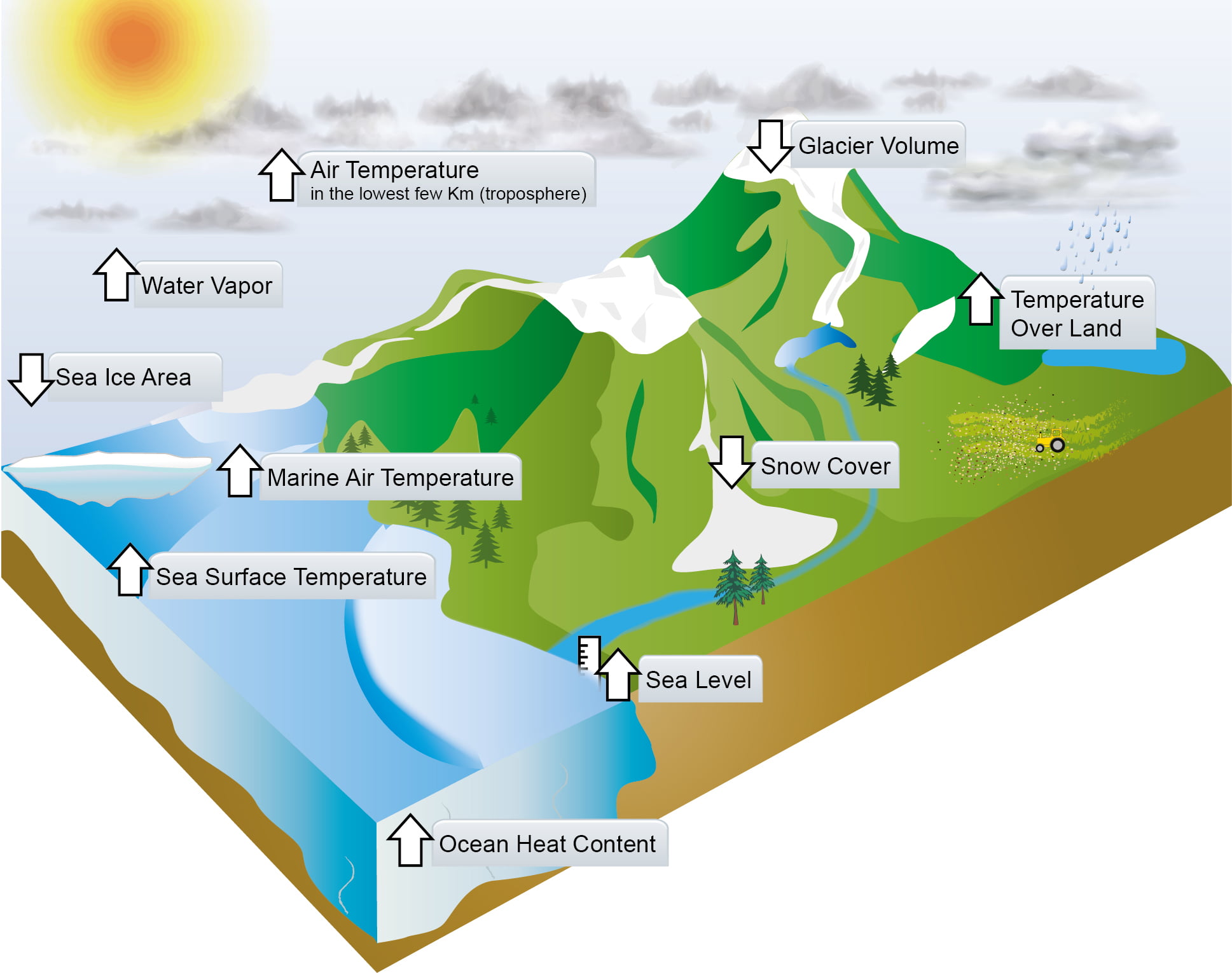
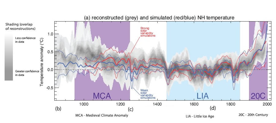
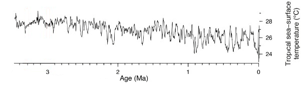
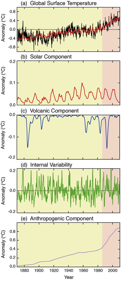

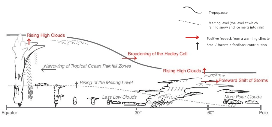
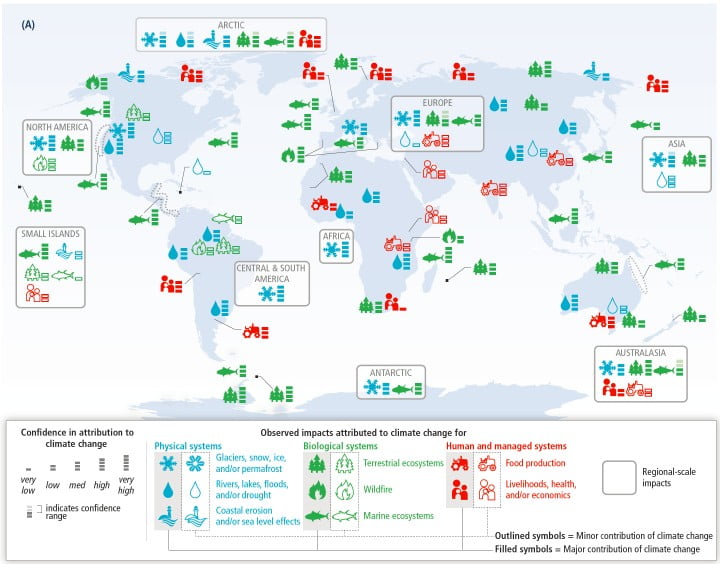

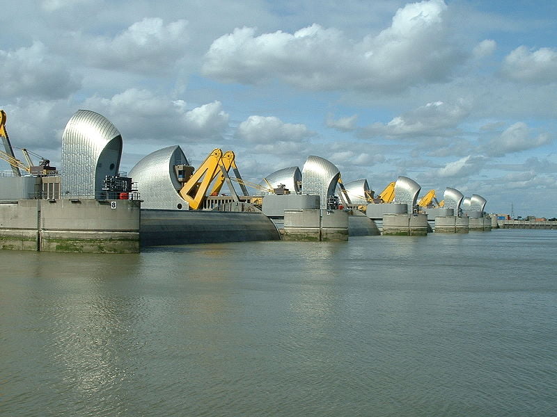


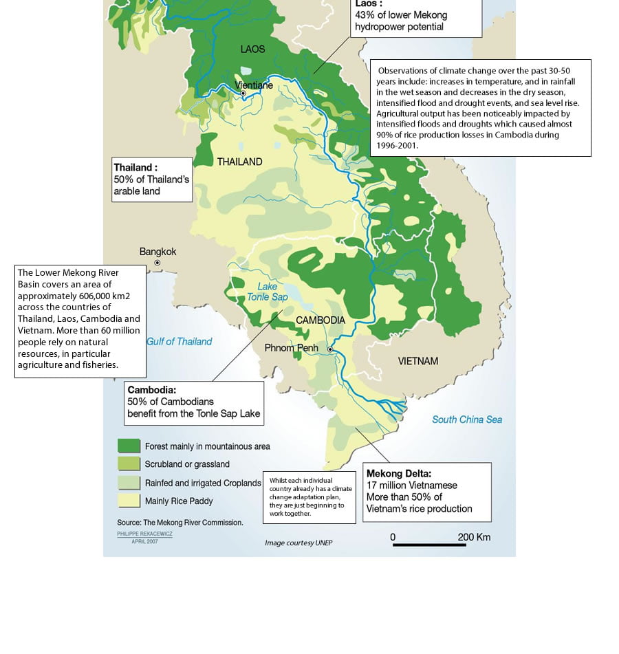
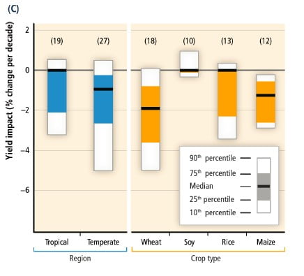
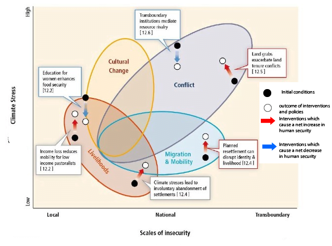


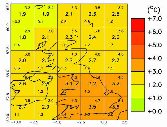
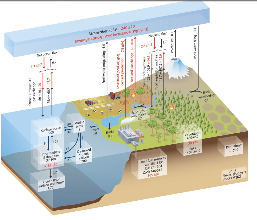

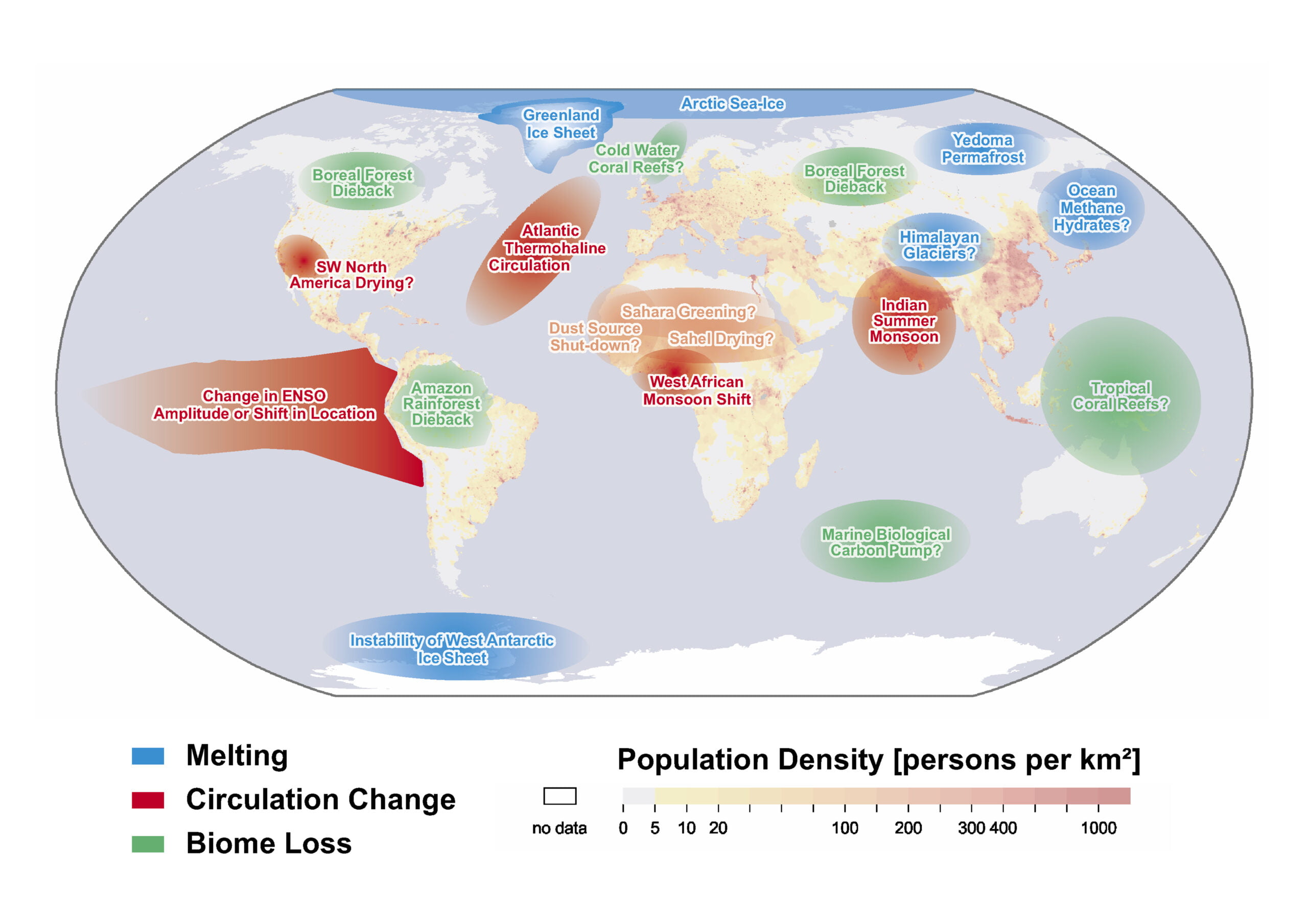
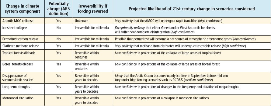
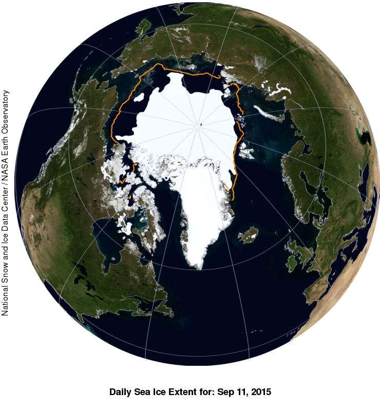


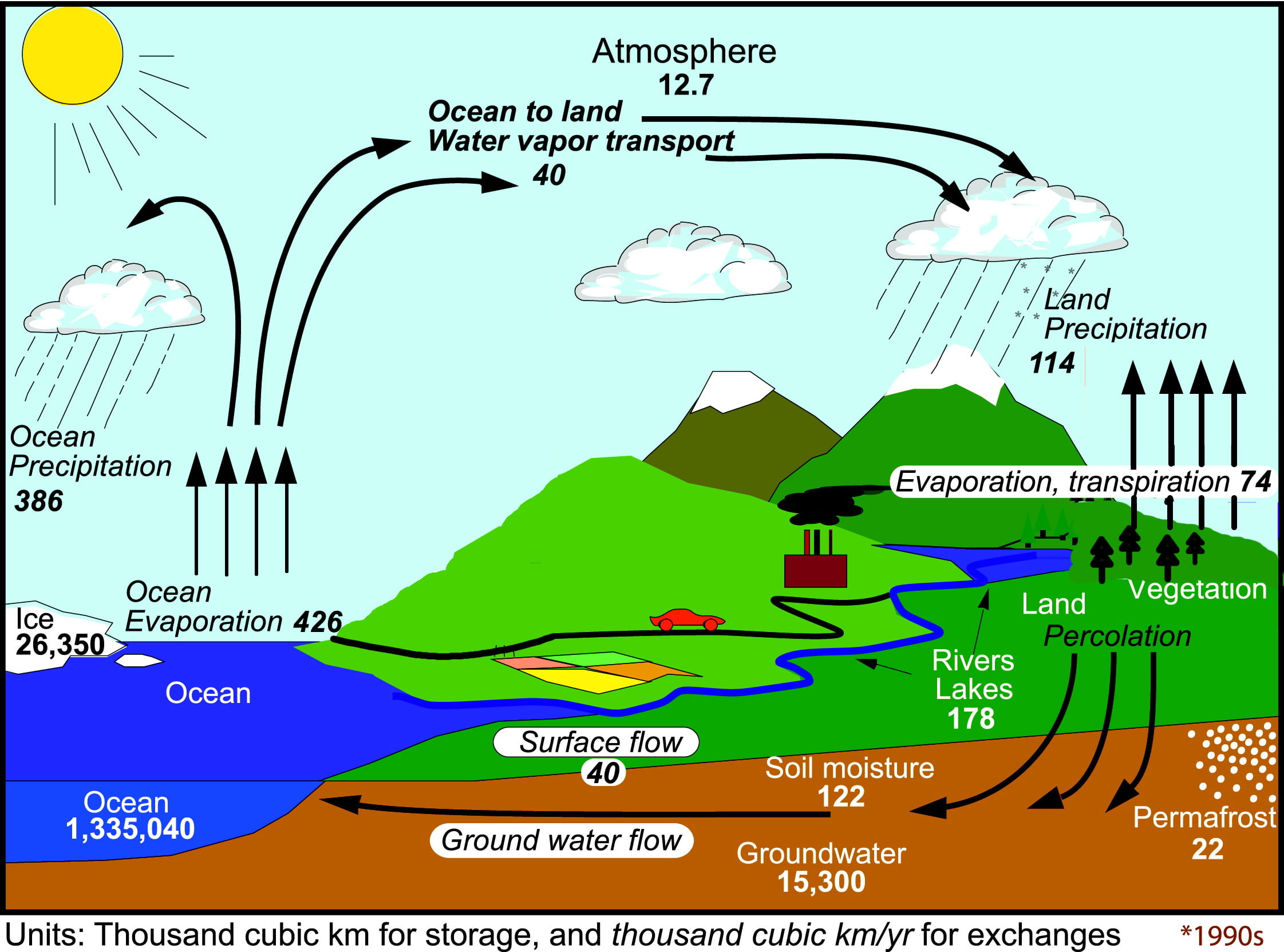
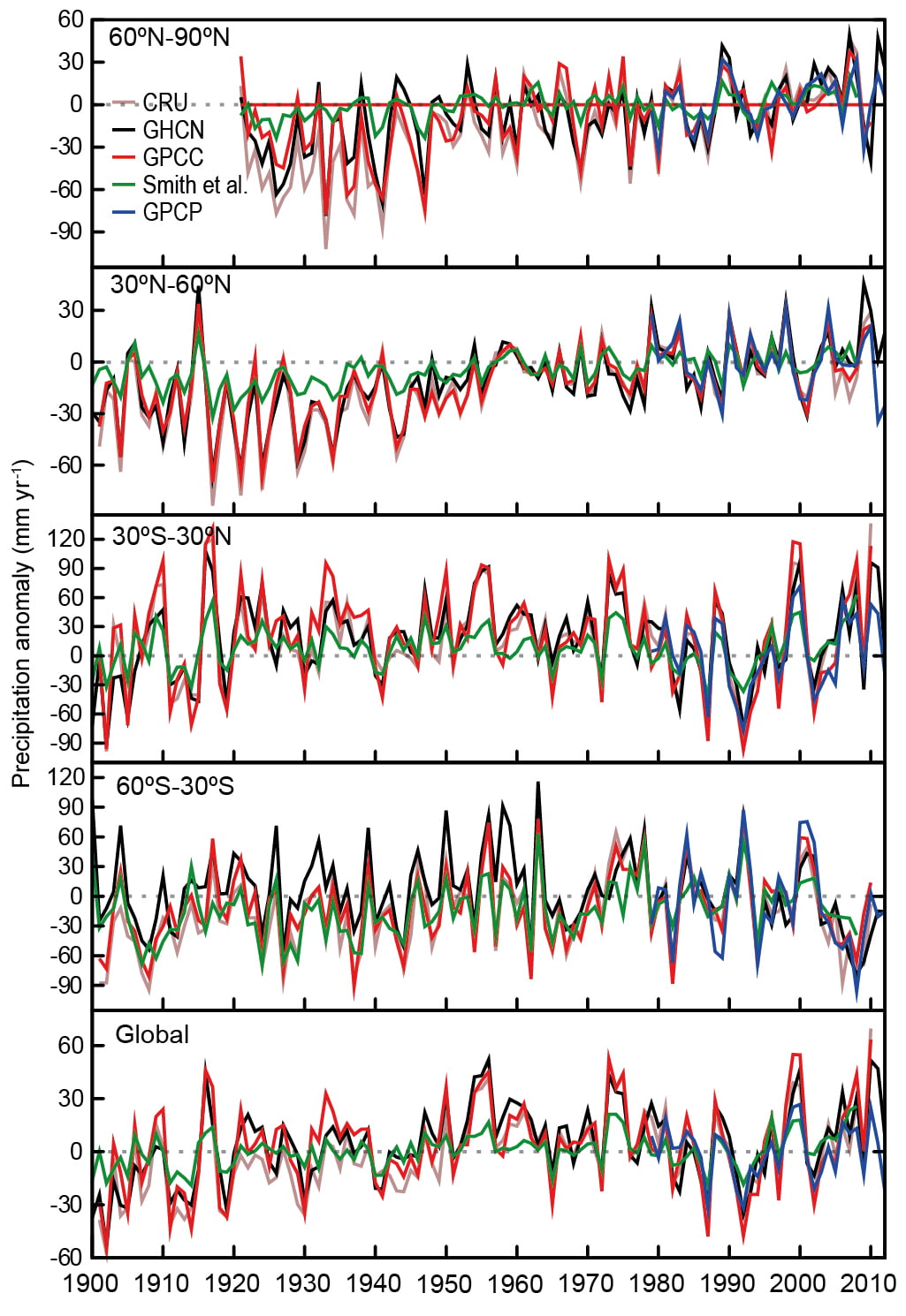
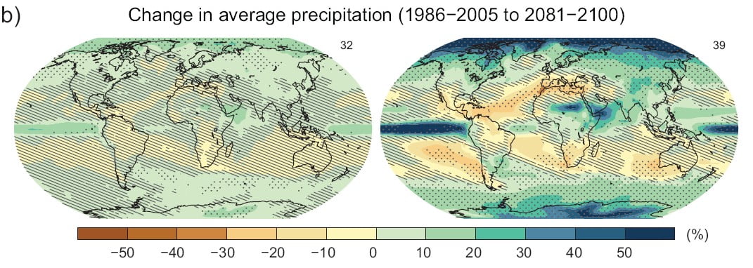
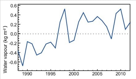
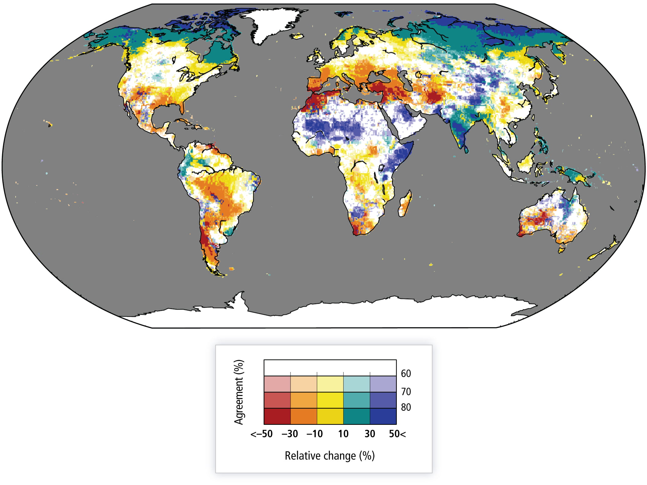
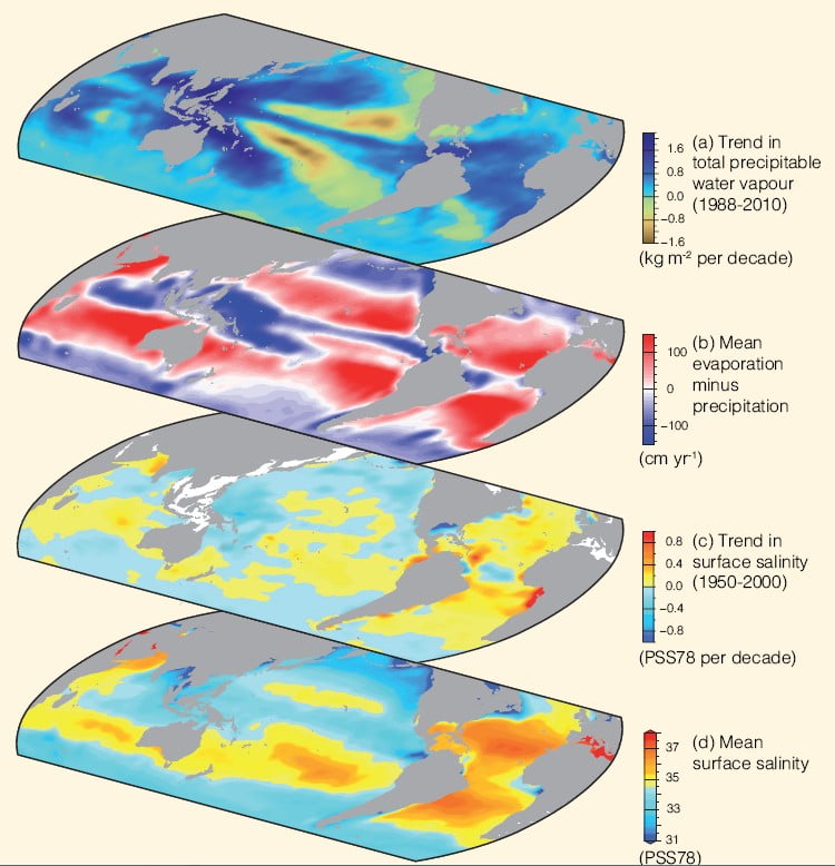
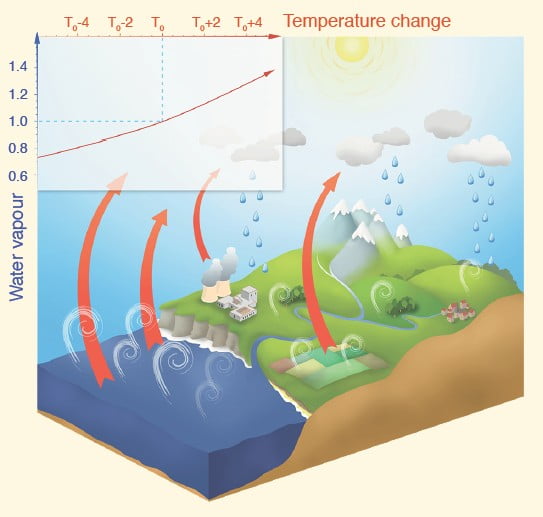
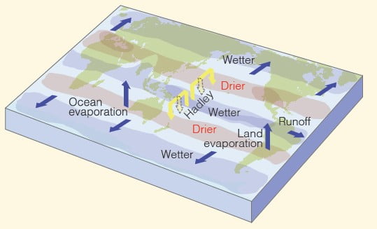
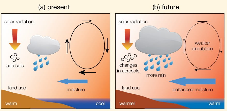
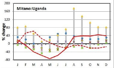
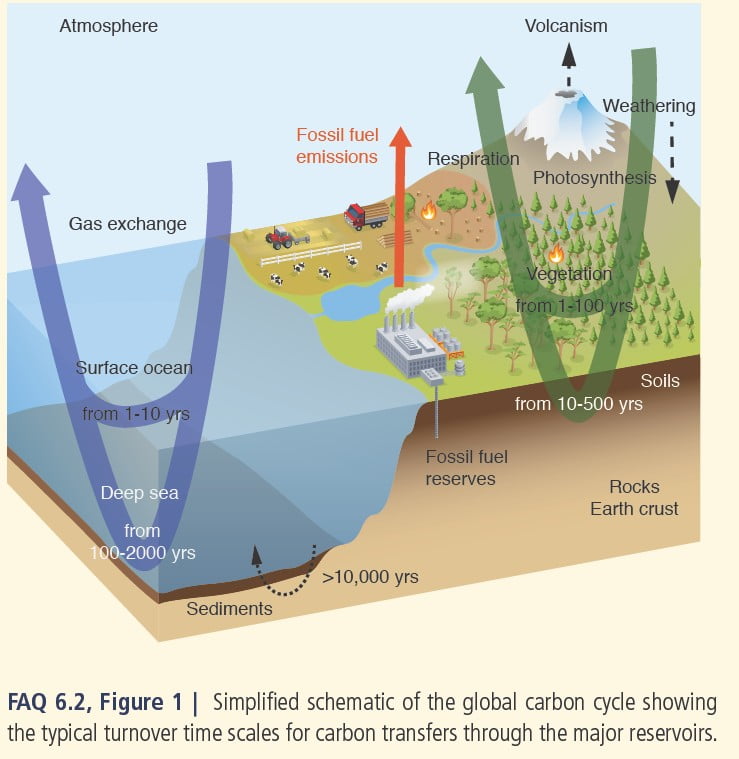

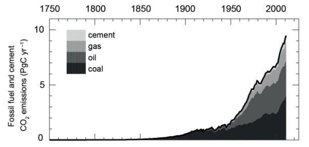
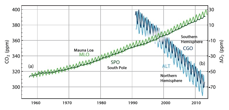
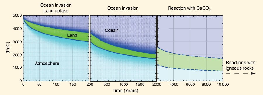
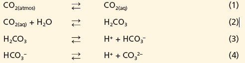
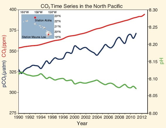
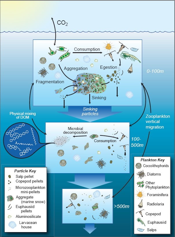
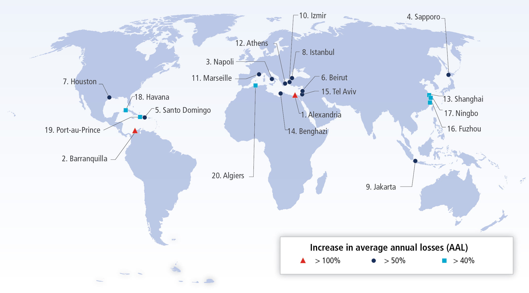
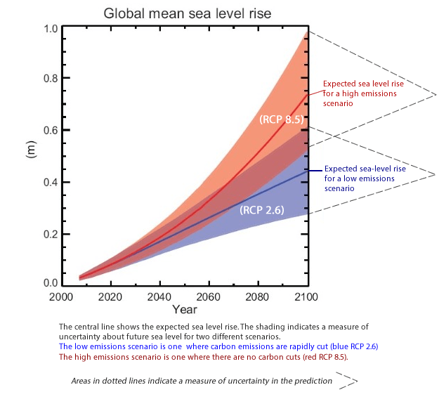
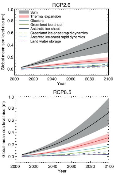
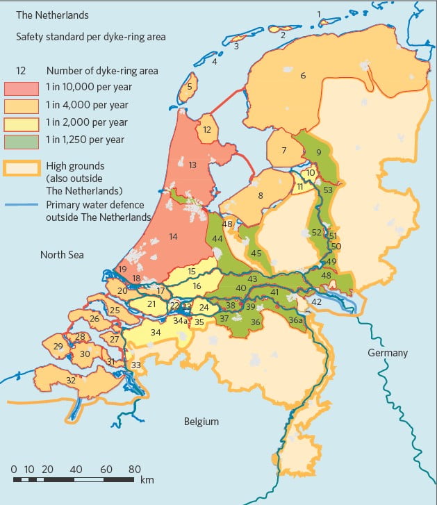
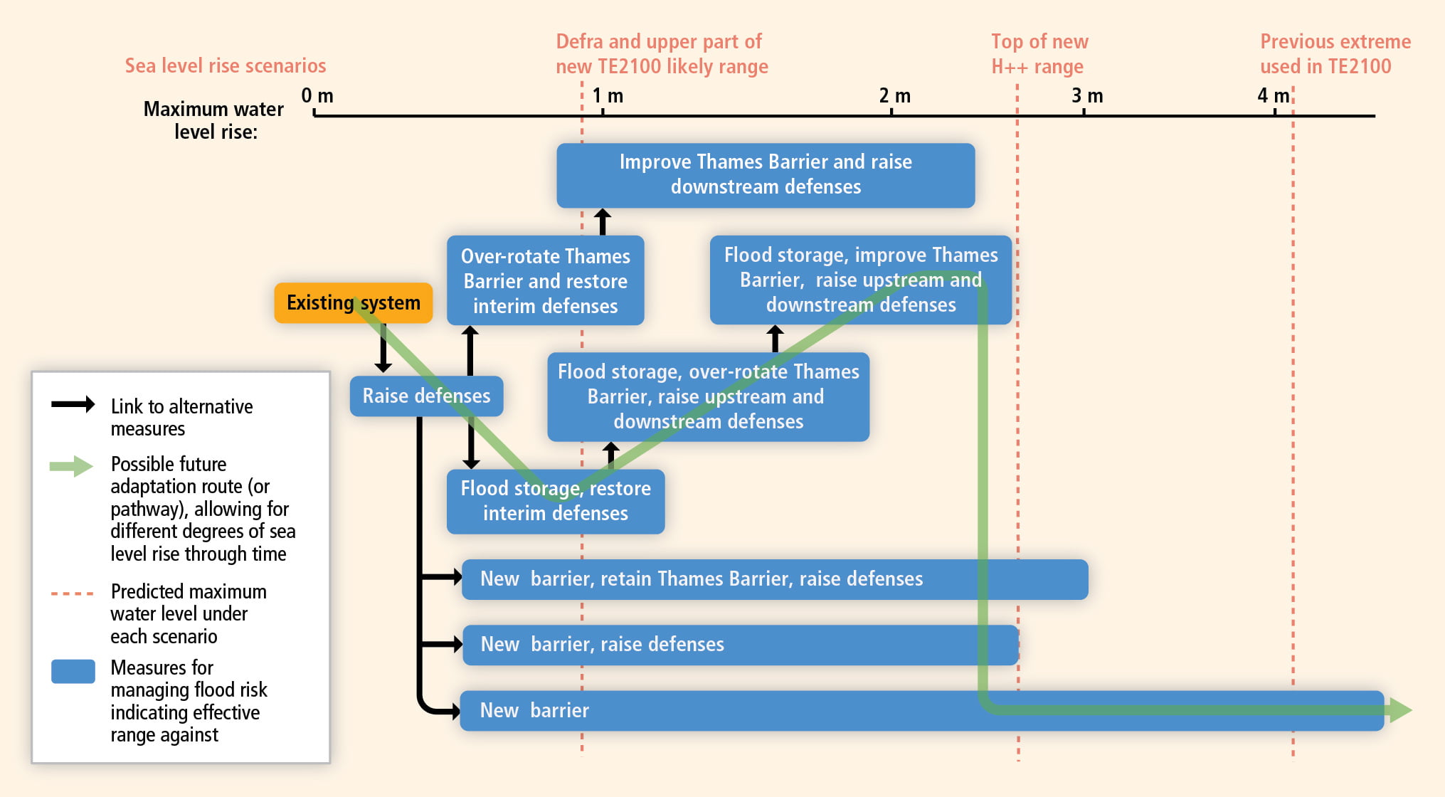

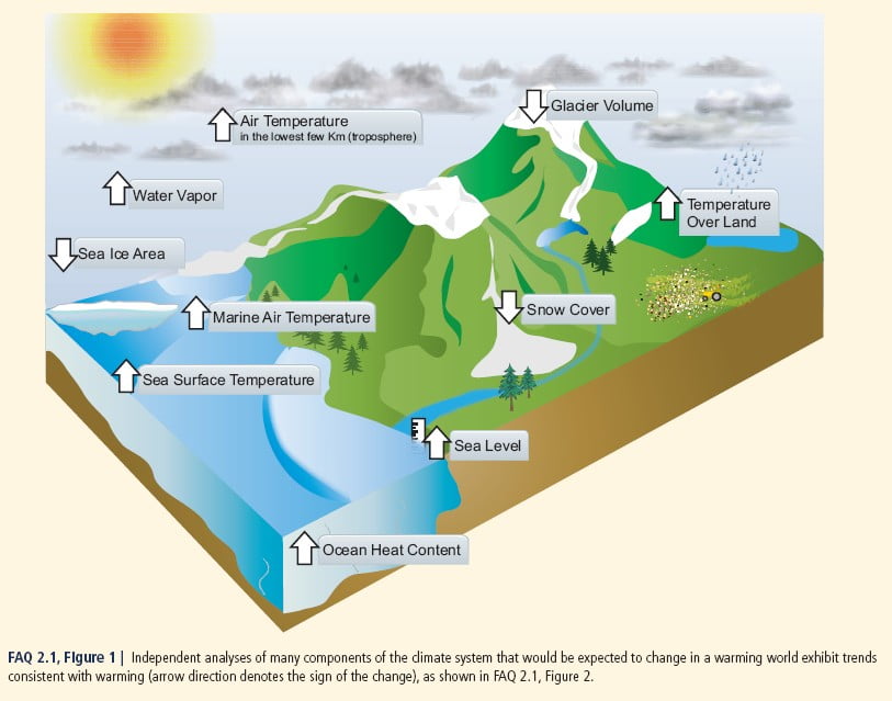
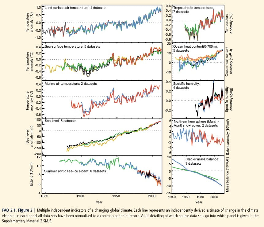
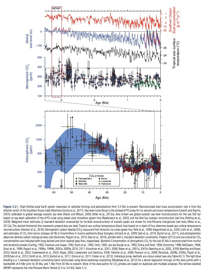
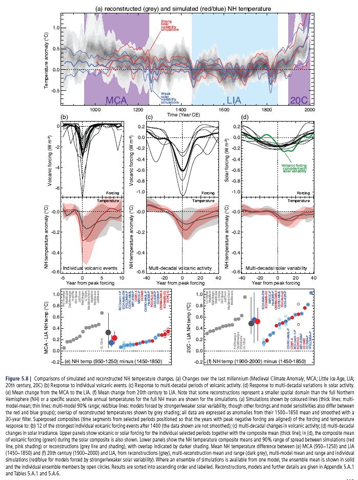
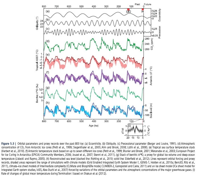
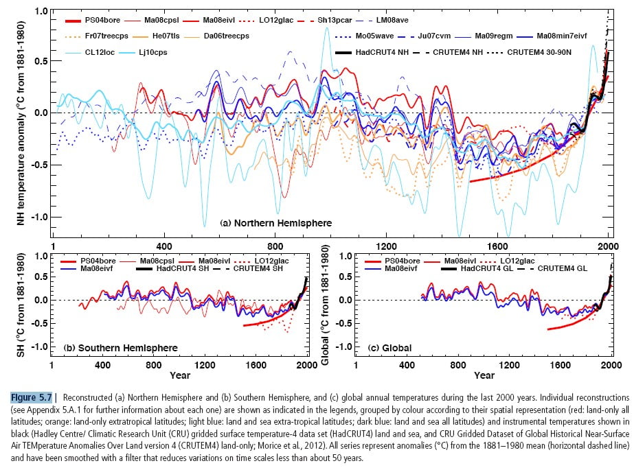
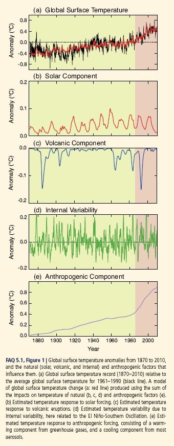
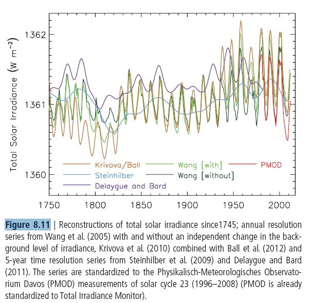
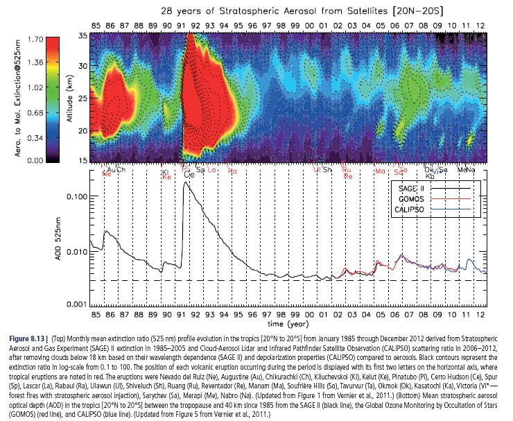
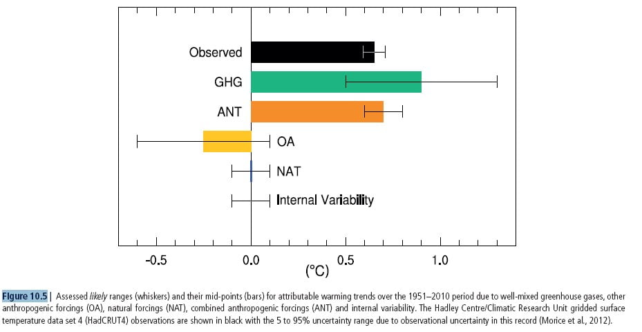
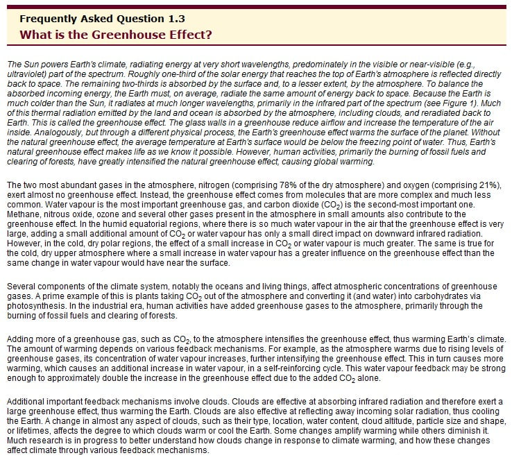
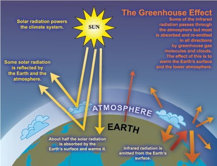
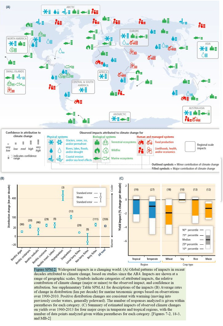
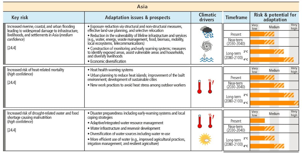
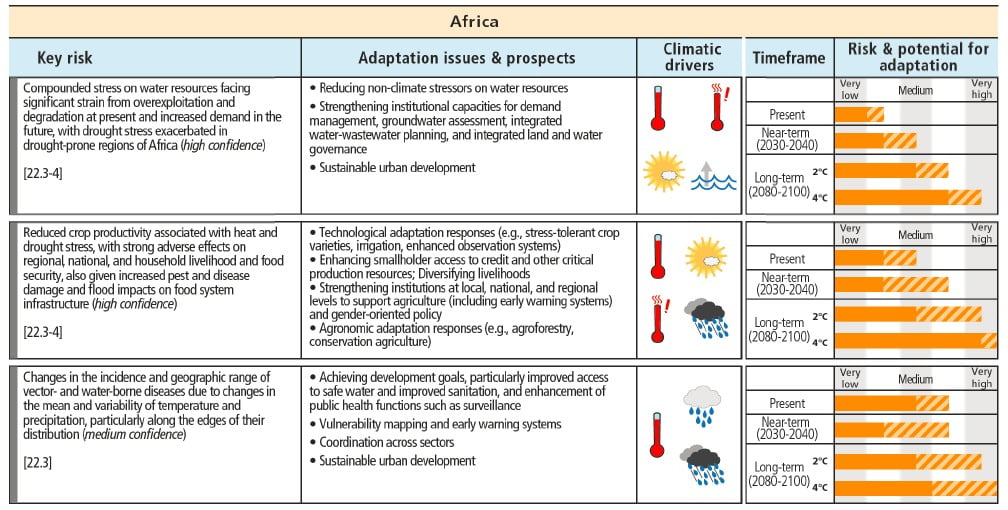
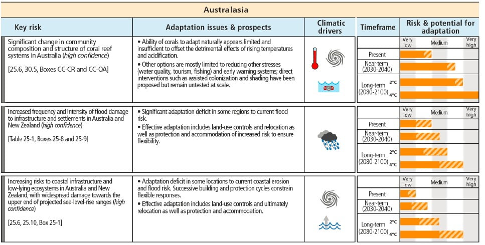
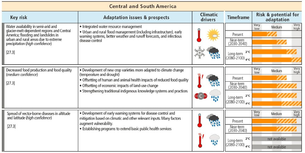
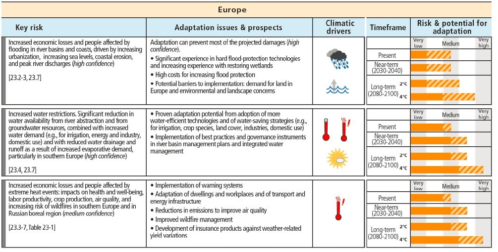
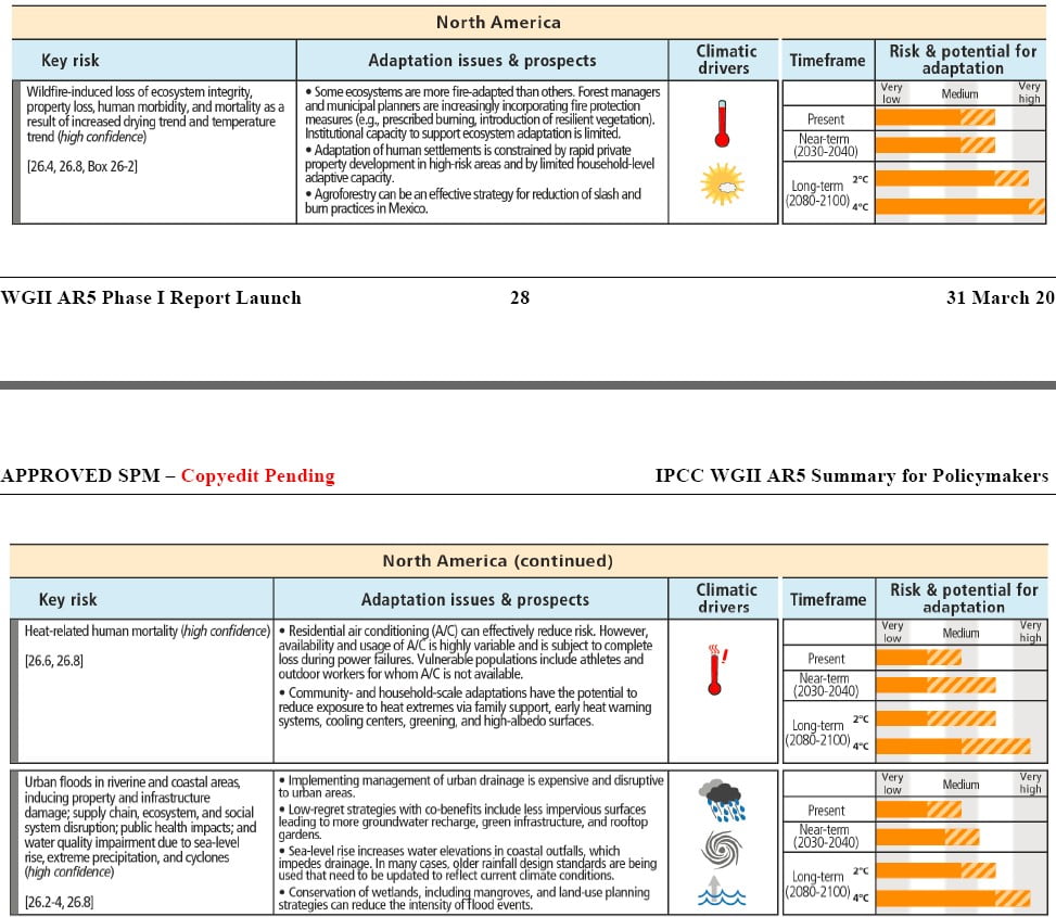
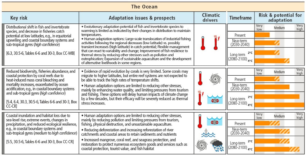
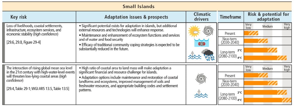
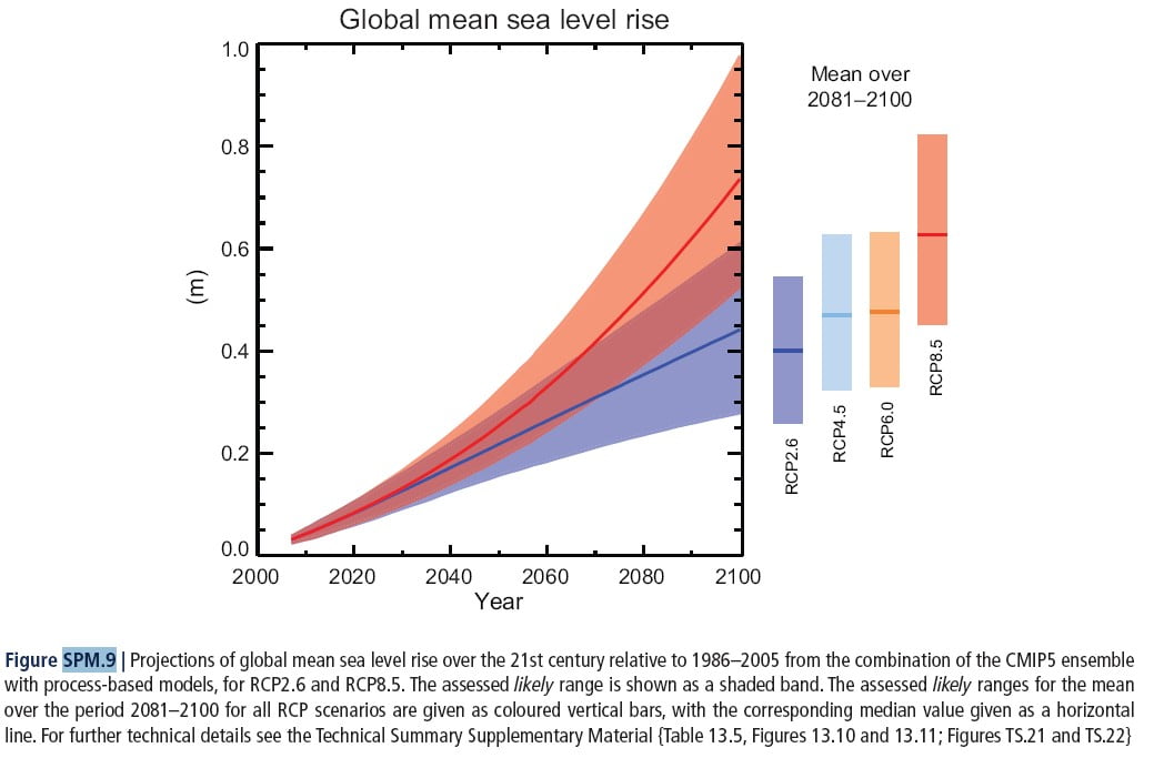
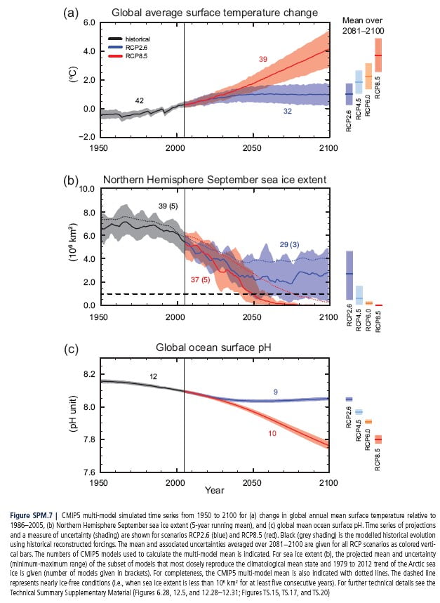
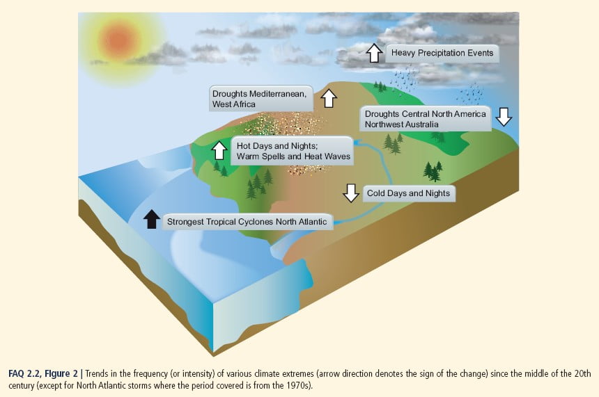
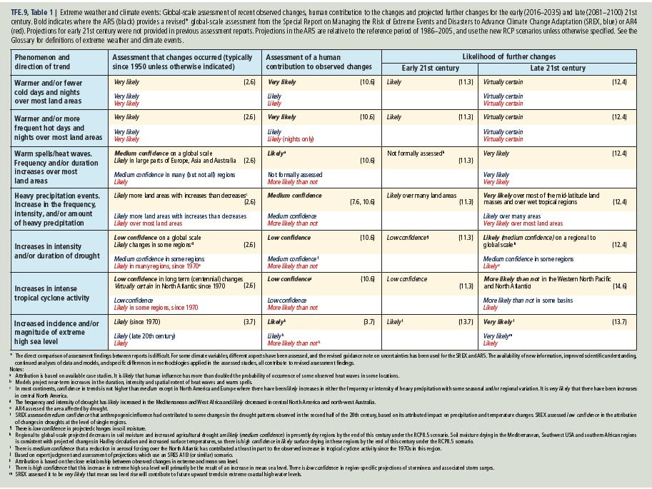
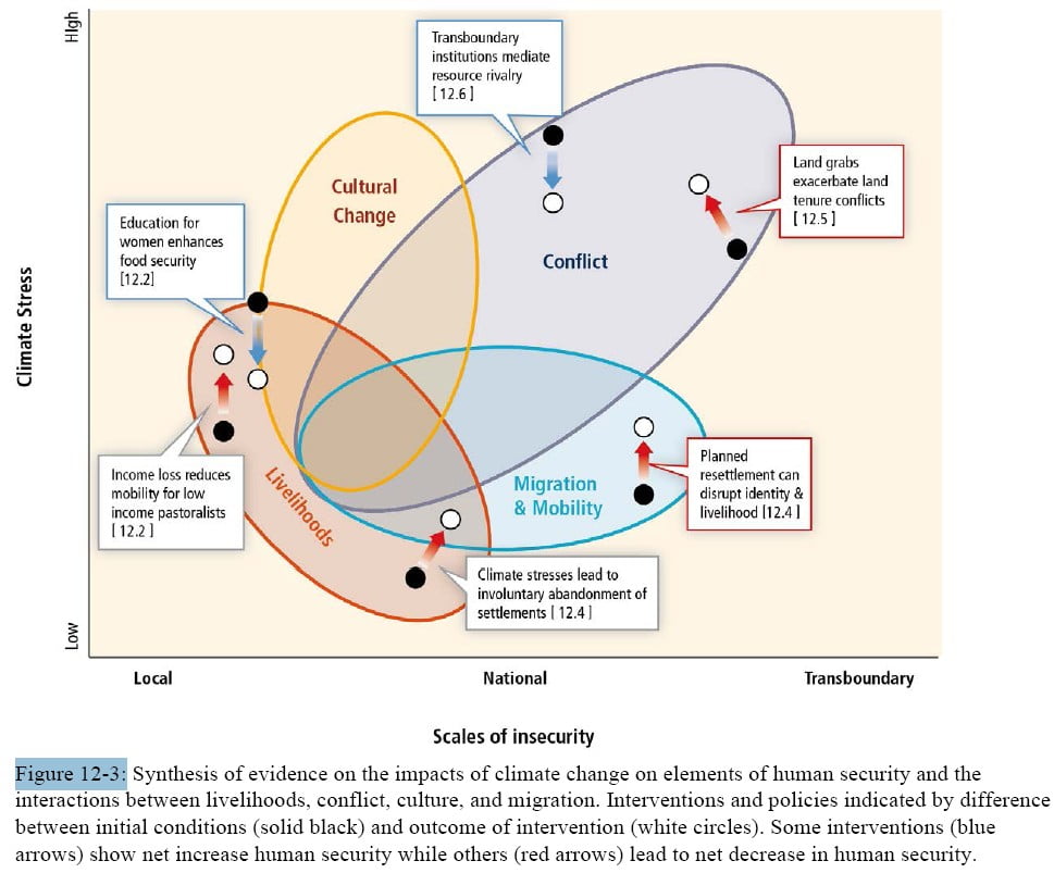