Age Range: 16 to 18

Case Studies

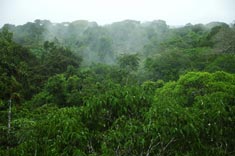
Vegetation changes in the Amazon basin

Return to main menu

Further Information

How do land-use and land-cover changes cause changes in climate?

What are the non-greenhouse gas effects of rising carbon dioxide on ecosystems?

The Carbon Dioxide fertilisation effect

A Possible Amazon Basin Tipping Point

In general, climate exerts a dominant control over the distribution of terrestrial vegetation and surface properties that in turn affects the local climate by changing the local atmospheric water, Carbon and energy budgets. It has been hypothesized that these vegetation–climate feedbacks can explain shifts of vegetation through time: Firstly, increased transpiration may result in more precipitation, which in turn increases plant productivity, which amplifies transpiration further. Secondly, increased productivity leads to more canopy cover, which is darker (lower albedo) than snow and bare soil. This results in higher temperatures on the above ground parts of individual plants, thus also amplifying plant productivity.

The combined effects of a warming climate, higher levels of CO₂, land-use change and increased Nitrogen availability may be responsible for primary productivity increases in many parts of the world. Enhanced productivity can lead to shifts in albedo and transpiration, which feed back to the water cycle through heat fluxes and precipitation.

Rising atmospheric CO₂ concentrations affect ecosystems directly including through biological and chemical processes such as the carbon dioxide fertilisation effect. Plants can respond to elevated CO₂ by opening their stomata less to take in the same amount of CO₂ or by structurally adapting their stomatal density and size, both potentially reducing transpiration which increases the water efficiency of the plants but reduces the flow of water vapour, and the energy that goes with it, to the atmosphere. Paleo records over the Late Quaternary (past million years) show that changes in the atmospheric CO₂ content between 180 and 280 ppmv had ecosystem-scale effects worldwide.

The direct effect of CO₂ on plant physiology, independent of its role as a greenhouse gas, means that assessing climate change impacts on ecosystems and hydrology solely in terms of global mean temperature rise is an oversimplification. A 2°C rise in global mean temperature, for example, may have a different net impact on ecosystems depending on the change in CO₂ concentration accompanying the rise: If a small change in CO₂ causes a 2°C rise, or, if other greenhouse gases are mainly responsible for the rise, the vegetation response will be different to a 2°C rise triggered by a large increase in CO₂.

Vegetation cover can be affected by climate change, with forest cover potentially decreasing (e.g. in the tropics) or increasing (e.g. in high latitudes). In particular, the Amazon forest has been the subject of several studies, generally agreeing that future climate change would increase the risk of tropical forest being replaced by seasonal forest or even savannah. The increase in atmospheric CO₂ reduces the risk, through an increase in the water efficiency of plants.

Direct human changes to the land cover can also have impacts on the carbon and water cycles, as well as on the Earth’s energy balance, through changes in surface albedo, transpiration and evaporation.

The coupling processes between terrestrial Carbon, Nitrogen and hydrological processes are extremely complex and far from well understood.

The effect of climate extremes on vegetation and the carbon and water cycles
Extreme events such as heatwaves, droughts and storms can cause vegetation death, fires and subsequent insect infestations which actually lead to a net output of carbon from ecosystems. For example, forests are characterized by the large biomass carbon stocks, which are vulnerable to wind damage, storms, ice storms, frost, drought, fire and pathogen or pest outbreaks.  Trees take a long time to regrow, so the recovery times for forest biomass lost through extreme events are particularly long. Therefore, the effects of climate extremes on the carbon balance in forests are both immediate and lagged, and potentially long-lasting. Climate extremes may also trigger processes that decrease the turnover rate of some carbon pools and lead to additional long-term sequestration in these pools. A well-known example is charcoal created in fires, which generally persists longer in soils than leaf litter.

During the European 2003 heatwave, it was the lack of precipitation (and soil moisture) rather than the high temperatures which was the main factor limiting vegetation growth in the temperate and Mediterranean forest ecosystems.

Further Links:

There is a nice, short summary article at http://www.carbonbrief.org/blog/2011/03/new-scientific-papers-on-plants-and-carbon-dioxide/
http://www.nature.com/nature/journal/v500/n7462/fig_tab/nature12350_F2.html An overview of how carbon flows may be triggered, or greatly altered, by extreme events including extreme precipitation.

Figure 1 from http://www.mdpi.com/1424-8220/9/11/8624/htm shows a schematic view of the components of the climate system, their processes and interactions.

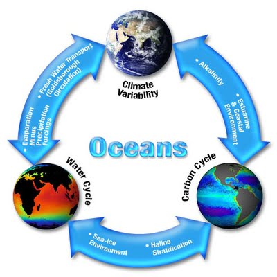
Ocean related feedback exists between climate variability, the water cycle and the carbon cycle.  http://nasa-information.blogspot.co.uk/2010/11/ocean-earth-system.html
http://www.nasa.gov/images/content/703470main_InfoGraphic.jpg  An infographic showing the limits to vegetation growth from soil nutrient availability.

A figure showing the ecosystem processes and feedbacks triggered by extreme climate events. http://www.nature.com/nature/journal/v500/n7462/fig_tab/nature12350_F1.html

How do land-use and land-cover changes cause changes in climate?
WG2 FAQ 4.1

Land use change affects the local as well as the global climate. Different forms of land cover and land use can cause warming or cooling and changes in rainfall, depending on where they occur in the world, what the preceding land cover was, and how the land is now managed. Vegetation cover, species composition and land management practices (such as harvesting, burning, fertilizing, grazing or cultivation) influence the emission or absorption of greenhouse gases. The brightness of the land cover affects the fraction of solar radiation that is reflected back into the sky, instead of being absorbed, thus warming the air immediately above the surface. Vegetation and land use patterns also influence water use and evapotranspiration, which alter local climate conditions. Effective land-use strategies can also help to mitigate climate change.

What are the non-greenhouse gas effects of rising carbon dioxide on ecosystems?
WG2 FAQ 4.2

Carbon dioxide (CO₂) is an essential building block of the process of photosynthesis. Simply put, plants use sunlight and water to convert CO₂ into energy. Higher CO₂ concentrations enhance photosynthesis and growth (up to a point), and reduce the water used by the plant. This means that water remains longer in the soil or recharges rivers and aquifers. These effects are mostly beneficial; however, high CO₂ also has negative effects, in addition to causing global warming. High CO₂ levels cause the nitrogen content of forest vegetation to decline and can increase their chemical defences, reducing their quality as a source of food for plant-eating animals. Furthermore, rising CO₂ causes ocean waters to become acidic, and can stimulate more intense algal blooms in lakes and reservoirs.

The Carbon Dioxide fertilisation effect
WG1 Box 6.3

Elevated atmospheric CO₂ concentrations lead to higher leaf photosynthesis and reduced canopy transpiration, which in turn lead to increased plant water use efficiency and reduced fluxes of latent heat from the surface to the atmosphere. The increase in leaf photosynthesis with rising CO₂, the so-called CO₂ fertilisation effect, plays a dominant role in terrestrial biogeochemical models to explain the global land carbon sink, yet it is one of most unconstrained process in those models.

Field experiments provide a direct evidence of increased photosynthesis rates and water use efficiency (plant carbon gains per unit of water loss from transpiration) in plants growing under elevated CO₂. These physiological changes translate into a broad range of higher plant carbon accumulation in more than two-thirds of the experiments and with increased net primary productivity (NPP) of about 20 to 25% at double CO₂ from pre-industrial concentrations. Since the last IPCC report, new evidence is available from long-term Free-air CO₂ Enrichment (FACE) experiments in temperate ecosystems showing the capacity of ecosystems exposed to elevated CO₂ to sustain higher rates of carbon accumulation over multiple years. However, FACE experiments also show the diminishing or lack of CO₂ fertilisation effect in some ecosystems and for some plant species. This lack of response occurs despite increased water use efficiency, also confirmed with tree ring evidence

Nutrient limitation is hypothesized as primary cause for reduced or lack of CO₂ fertilisation effect observed on NPP in some experiments. Nitrogen and phosphorus are very likely to play the most important role in this limitation of the CO₂ fertilisation effect on NPP, with nitrogen limitation prevalent in temperate and boreal ecosystems, and phosphorus limitation in the tropics. Micronutrients interact in diverse ways with other nutrients in constraining NPP such as molybdenum and phosphorus in the tropics. Thus, with high confidence, the CO₂ fertilisation effect will lead to enhanced NPP, but significant uncertainties remain on the magnitude of this effect, given the lack of experiments outside of temperate climates.

A Possible Amazon Basin Tipping Point
WG2 Box 4.3

Since the last assessment report of the IPCC (AR4), our understanding of the potential of a large-scale, climate-driven, self-reinforcing transition of Amazon forests to a dry stable state (known as the Amazon “forest dieback”) has improved. Modelling studies indicate that the likelihood of a climate-driven forest dieback by 2100 is lower than previously thought, although lower rainfall and more severe drought is expected in the eastern Amazon. There is now medium confidence that climate change alone (that is, through changes in the climate envelope, without invoking fire and land use) will not drive large-scale forest loss by 2100 although shifts to drier forest types are predicted in the eastern Amazon.

Meteorological fire danger is projected to increase. Field studies and regional observations have provided new evidence of critical ecological thresholds and positive feedbacks between climate change and land-use activities that could drive a fire mediated, self-reinforcing dieback during the next few decades. There is now medium confidence that severe drought episodes, land use, and fire interact synergistically to drive the transition of mature Amazon forests to low-biomass, low-statured fire-adapted woody vegetation. Most primary forests of the Amazon Basin have damp fine fuel layers and low susceptibility to fire, even during annual dry seasons. Forest susceptibility to fire increases through canopy thinning and greater sunlight penetration caused by tree mortality associated with selective logging, previous forest fire, severe drought, or drought-induced tree mortality. The impact of fire on tree mortality is also weather-dependent. Under very dry, hot conditions, fire-related tree mortality can increase. Under some circumstances, tree damage is sufficient to allow light-demanding, flammable grasses to establish in the forest understorey, increasing forest susceptibility to further burning. There is high confidence that logging, severe drought, and previous fire increase Amazon forest susceptibility to burning. Landscape level processes further increase the likelihood of forest fire. Fire ignition sources are more common in agricultural and grazing lands than in forested landscapes, and forest conversion to grazing and crop lands can inhibit regional rainfall through changes in albedo and evapotranspiration or through smoke that can inhibit rainfall under some circumstances. Apart from these landscape processes, climate change could increase the incidence of severe drought episodes.

If recent patterns of deforestation (through 2005), logging, severe drought, and forest fire continue into the future, more than half of the region’s forests will be cleared, logged, burned or exposed to drought by 2030, even without invoking positive feedbacks with regional climate, releasing 20±10 Pg of carbon to the atmosphere. The likelihood of a tipping point being reached may decline if extreme droughts (such as 1998, 2005, and 2010) become less frequent, if land management fires are suppressed, if forest fires are extinguished on a large scale, if deforestation declines, or if cleared lands are reforested. The 77% decline in deforestation in the Brazilian Amazon with 80% of the region’s forest still standing demonstrates that policy-led avoidance of a fire-mediated tipping point is plausible.

WG2 Chapter 4, Figure 8.
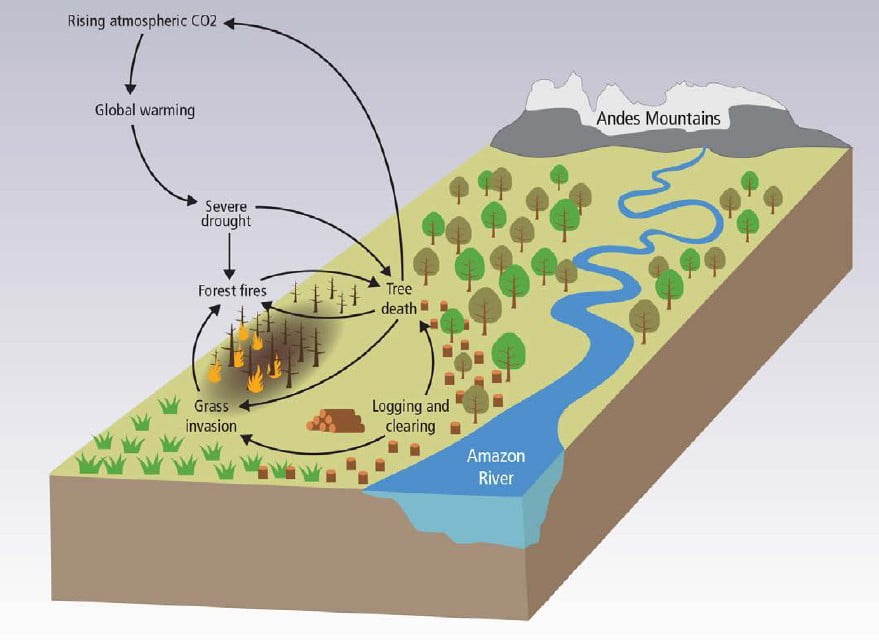
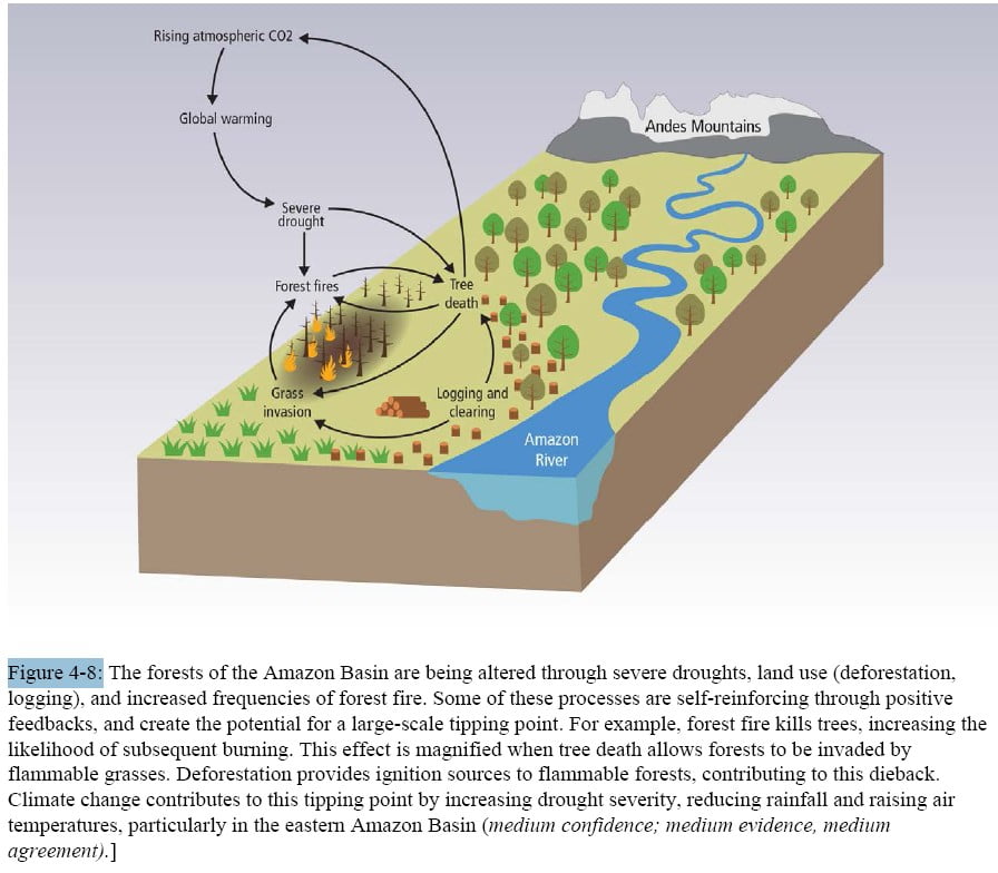
The forests of the Amazon Basin are being altered through severe droughts, land use (deforestation, logging), and increased frequencies of forest fire. Some of these processes are self-reinforcing through positive feedbacks, and create the potential for a large-scale tipping point. For example, forest fire kills trees, increasing the likelihood of subsequent burning. This effect is magnified when tree death allows forests to be invaded by grasses, which are more flammable. Deforestation provides ignition sources to flammable forests, contributing to this dieback. Climate change contributes to this tipping point by increasing drought severity, reducing rainfall and raising air temperatures, particularly in the eastern Amazon Basin.

Vegetation changes in the Amazon basin

WG2 Chapter 4, Figure 8. The forests of the Amazon Basin are already being altered through severe droughts, changes in land use (deforestation, logging), and increased frequencies of forest fire. Some of these processes are self-reinforcing through positive feedbacks, and create the potential for a large-scale tipping point. For example, forest fire kills trees, increasing the likelihood of subsequent burning. This effect is magnified when tree death allows forests to be invaded by flammable grasses. Deforestation provides ignition sources to flammable forests, contributing to this dieback. Climate change contributes to this tipping point by increasing drought severity, reducing rainfall and raising air temperatures, particularly in the eastern Amazon Basin.

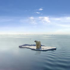
There is a high risk that the large magnitudes and high rates of climate change this century will result in abrupt and irreversible regional-scale changes to terrestrial and freshwater ecosystems, especially in the Amazon and Arctic, leading to additional climate change.

There are plausible mechanisms, supported by experimental evidence, observations, and climate model simulations, for the existence of ecosystem tipping points in the rainforests of the Amazon basin. Climate change (temperature and precipitation changes) alone is not projected to lead to abrupt widespread loss of forest cover in the Amazon during this century. However, a projected increase in severe drought episodes, related to stronger El Niño events, together with land-use change and forest fires, would cause much of the Amazon forest to transform to less dense, drought- and fire-adapted ecosystems. This would risk reducing biodiversity in an important ecosystem, and would reduce the amount of carbon absorbed from the atmosphere through photosynthesis. It would also reduce the amount of evaporation, increasing the warming locally. Large reductions in deforestation, as well as wider application of effective wildfire management would lower the risk of abrupt change in the Amazon.

Amazonian forests were estimated to have lost 1.6 PgC and 2.2 PgC following the severe droughts of 2005 and 2010, respectively.

A Possible Amazon Basin Tipping Point